PADP 7120 Data Applications in PA

class: center, middle, inverse, title-slide

.title[
# PADP 7120 Data Applications in PA
]
.subtitle[
## RLab 7: Data Viz 2
]
.author[
### Alex Combs
]
.institute[
### UGA | SPIA | PADP
]
.date[
### Last updated: October 24, 2022
]

---

# Objectives

- Incorporate the data we combined in previous RLab to generate more accurate graphs

- Cover a few more ways to improve graphs

---
# Setup

> **Open the same project and Rmd we have worked on the last two labs. No need to start a new project**

> **Change yesterday to the correct date.**

> **Rerun all the code up to the point where you have the `covid_ga` dataset that now includes county population.**

---
# Adjusting for Population

- We realized that it is misleading to compare counts of COVID cases and/or deaths across counties of different populations

- We need to compute counts per capita or some standard number of people, such as 100,000

- And create two **normalized** variables, `cases_rate`, `deaths_rate`.

---
# Adjusting for Population

- Our population variable is in single units.

- First, could create a new variable for population in 100,000s. How?

- Then, we need to create cases and deaths per 100,000. How?

---
# Adjusting for Population

> **Insert a new code chunk below the left join that added population to `covid_ga`. Overwrite `covid_ga`, creating three new variables: `pop100thou`, `cases_rate`, and `deaths_rate`.**

```r
covid_ga <- ___ %>% 
  ___(pop100thou = ___,
         cases_rate = ___, 
         deaths_rate = ___)
```

---
# Common Viz Adjustments

- Non-data ink
  - ~~Labels (title and axes)~~
  - ~~Themes~~
  - Axes & scales (tick marks, commas, dollars, log scale)

- Geometric object adjustments
  - Color
  - Shape/line type & size
  - Reference lines

---
# Viz 1

> **Improve Viz1 by adding a title and labels as well as change the theme to one of R's default themes**

```r
covid_ga %>% 
  filter(date == yesterday) %>% 
  ggplot(aes(x = cases)) +
  geom_histogram()
```

![](rlab7-polished-viz_files/figure-html/unnamed-chunk-7-1.png)

---
# Viz 1 - Labels and Themes

```r
covid_ga %>% 
  filter(date == yesterday) %>% 
  ggplot(aes(x = cases)) +
  geom_histogram() +
* labs(title = 'Total COVID Cases in GA Counties',
*      x = 'Total Cases',
*      y = 'Counties') +
* theme_minimal()
```

---
# Viz 1 - Labels and Themes

![](rlab7-polished-viz_files/figure-html/unnamed-chunk-9-1.png)

---
# Viz 1 - Log scale

- The right skew bunches most counties within a small interval that is difficult to distinguish.

> **Correct the skew by converting the x axis to log scale**

```r
covid_ga %>% 
  filter(date == yesterday) %>% 
  ggplot(aes(x = cases)) +
  geom_histogram() +
  labs(title = 'Total COVID Cases in GA Counties',
       x = 'Total Cases',
       y = 'Counties') +
* scale_x_log10() +
  theme_minimal()
```

---
# Viz 1 - Log scale

![](rlab7-polished-viz_files/figure-html/unnamed-chunk-11-1.png)

---
# Viz 1 - Fill and outline

> **Change the `fill` color and outline `color` of the histogram**

```r
covid_ga %>% 
  filter(date == yesterday) %>% 
  ggplot(aes(x = cases)) +
* geom_histogram(fill = 'steelblue', color = 'white') +
  labs(title = 'Total COVID Cases in GA Counties',
       x = 'Total Cases',
       y = 'Counties') +
  scale_x_log10() +
  theme_minimal()
```

---
# Viz 1 - Fill and outline

![](rlab7-polished-viz_files/figure-html/unnamed-chunk-13-1.png)

---
# Viz 1 - Adding Comma Separator

> **Use the code below to display x axis in comma format.**

```r
covid_ga %>% 
  filter(date == yesterday) %>% 
  ggplot(aes(x = cases)) +
  geom_histogram(fill = 'steelblue', color = 'white') +
  labs(title = 'Total COVID Cases in GA Counties',
       x = 'Total Cases',
       y = 'Counties') +
* scale_x_log10(labels = scales::label_comma()) +
  theme_minimal()
```

---
# Viz 1 - Adding Comma Separator

![](rlab7-polished-viz_files/figure-html/unnamed-chunk-15-1.png)

---
# Viz 1 - Change text size

```r
covid_ga %>% 
  filter(date == yesterday) %>% 
  ggplot(aes(x = cases)) +
  geom_histogram(fill = 'steelblue', color = 'white') +
  labs(title = 'Total COVID Cases in GA Counties',
       x = 'Total Cases',
       y = 'Counties') +
  scale_x_log10(labels = scales::label_comma()) +
  theme_minimal() +
* theme(title = element_text(size = 16),
*       axis.text = element_text(size = 12))
```

---
# Viz 1 - Change text size

![](rlab7-polished-viz_files/figure-html/unnamed-chunk-17-1.png)

---
# Viz 2

> **On your own, make similar adjustments to the histogram of total county deaths**

---
# Viz 2

![](rlab7-polished-viz_files/figure-html/unnamed-chunk-18-1.png)

---
# Viz 3

.pull-left[
![](rlab7-polished-viz_files/figure-html/unnamed-chunk-19-1.png)
]

.pull-right[
- Y axis isn't interpretable.
- We can remove the tick marks, line, and text for the y axis
]

---
# Viz 3: Remove axis elements

> **Add below code to remove parts of graph**

```r
covid_ga %>% 
  filter(date == yesterday) %>%
  ggplot(aes(x = deaths)) +
  geom_boxplot() +
* theme(axis.ticks.y = element_blank(),
*       axis.line.y = element_blank(),
*       axis.text.y = element_blank())
```

---
# Viz 3: Remove axis elements

![](rlab7-polished-viz_files/figure-html/unnamed-chunk-21-1.png)

---
# Viz 3: Change theme and fill color

> **On your own, try to change the theme and fill color of the box plot. Add a title, subtitle that specifies the date, and improve the axis label. Similar to the graph below.**

![](rlab7-polished-viz_files/figure-html/unnamed-chunk-22-1.png)

---
# Viz 3: Change theme and fill color

```r
covid_ga %>% 
  filter(date == yesterday) %>%
  ggplot(aes(x = deaths)) +
* geom_boxplot(fill = 'springgreen4') +
* labs(title = 'Total County COVID Deaths',
*      subtitle = 'October 23, 2022', x = 'Total Deaths') +
* theme_classic() +
  theme(axis.ticks.y = element_blank(),
        axis.line.y = element_blank(),
        axis.text.y = element_blank())
```

---
# Viz 3: Change figure size and alignment

- Figure size and alignment is controlled via code chunk options

> **Add the following code chunk options to viz 3.**

```r
{r viz3, fig.width=5, fig.height=3, fig.align='center'}
```

- This will change the size to 5in wide and 3in tall and center its position when knit

![](rlab7-polished-viz_files/figure-html/unnamed-chunk-25-1.png)

---
# Selected Counties

- Now rerun the code that created `covid_ga_5`

```r
ga_counties <- c('Fulton', 'Cobb', 'DeKalb', 'Gwinnett', 'Clarke')

covid_ga_5 <- covid_ga %>% 
  filter(county %in% ga_counties)
```

---
# Viz 4

> **Update the bar graph comparing our 5 chosen counties using cases per 100,000**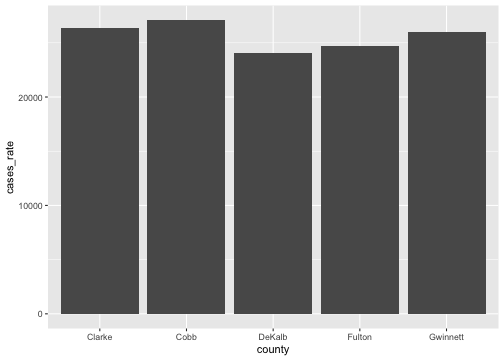

![](rlab7-polished-viz_files/figure-html/unnamed-chunk-27-1.png)

---
# Viz 4

```r
covid_ga_5 %>% 
  filter(date == yesterday) %>% 
* ggplot(aes(x = county, y = cases_rate)) +
  geom_col()
```

---
# Viz 4: Reorder bars

- Generally preferable to have bars in ascending or descending order

> **Add the following code**

```r
covid_ga_5 %>% 
  filter(date == yesterday) %>% 
* ggplot(aes(x = reorder(county, -cases_rate), y = cases_rate)) +
  geom_col()
```

---
# Viz 4: Reorder bars

![](rlab7-polished-viz_files/figure-html/unnamed-chunk-30-1.png)

---
# Viz 4: Other Adjustments

- We could make similar adjustments as before to improve the look

![](rlab7-polished-viz_files/figure-html/unnamed-chunk-31-1.png)

---
# Viz 7

> **Update first line graph to use cases per 100,000 people.**

![](rlab7-polished-viz_files/figure-html/unnamed-chunk-32-1.png)

---
# Exporting a graph as a separate file

- Anytime we run code that makes a graph, R stores it in memory in case we want to export it.

- Following code will save our last graph

```r
ggsave("covid_ga_case_trends.png", width = 8, height = 6)
```

- Can export as .jpeg, .tiff, .eps, .pdf, and more

---
# Changing how dates are displayed

- Suppose we want the x axis to display the full name of every other month

> **Add the following to Viz 7.**

```r
covid_ga_5 %>%
  ggplot(aes(x = date, y = cases_rate, color = county)) +
  geom_line() +
* scale_x_date(date_breaks = '2 month',
*              labels = scales::date_format('%B')) +
  labs(title = 'Total COVID Cases Among Selected Georgia Counties',
       x = '',
       y = 'Cases per 100,000',
       color = 'County') +
  theme_minimal() +
  theme(axis.text=element_text(size=12),
        title = element_text(size=12))
```

![](rlab7-polished-viz_files/figure-html/unnamed-chunk-34-1.png)

---
# Adding Reference Lines

- Suppose we want to provide a visual marker for the beginning of UGA's Fall 2022 semester.

> **Add the following to Viz 7.**

```r
  geom_vline(xintercept = as.Date('2022-08-15'),
             color = 'black', linetype = 'dashed')
```

---
# Adding Reference Lines

![](rlab7-polished-viz_files/figure-html/unnamed-chunk-36-1.png)

---
# Viz 8

> **Make similar adjustments to the line graph displaying deaths per 100,000**

![](rlab7-polished-viz_files/figure-html/unnamed-chunk-37-1.png)

---
class: inverse, middle, center

# The rank of county cases is not the same as the rank of county deaths. Why?

---
# Upload Rmd

> **Knit your Rmd. Upload Rmd to eLC.**