10 Sampling
“This is what I’m learning, at 82 years old: the main thing is to be in love with the search for truth.”
—Maya Angelou
We now turn our attention to inference, which involves taking a sample from a population to make conclusions about the population with some degree of certainty. At its foundation, inference is about the search for truth. Specifically, when we calculate some estimate using a sample of data, we use inference to say whether that estimate is a good guess of the unobserved population parameter. Rather than focus on sampling techniques (e.g. random, clustered, stratified, convenience), this chapter focuses on the theory that allows us to use samples for inference as well as the potential limitations of doing so.
10.1 Learning objectives
- Explain the 68-95-99 rule and apply it given the mean and standard deviation of a normal distribution
- Explain how a sampling distribution is constructed
- Explain why the Central Limit Theorem is needed to conduct inferential statistics and how it allows us to do so
- Given an estimate and standard error, construct 95 and 99 percent confidence intervals
- Interpret confidence intervals
- Explain the effect of random or biased sampling on the accuracy and precision of a sample estimate and sampling distribution
- Explain the effect of sample size on the accuracy and precision of a sample estimate and sampling distribution
10.2 Normal distribution
When we calculate an estimate, the estimate is highly unlikely to be exactly equal to the population parameter it is intended to represent. But, given a sample and an estimate, we can calculate the range in which the parameter falls with a certain degree of confidence. If that range does not include zero, then we have reason to believe the parameter is positive or negative. A non-zero parameter may be cause for action. Or, depending on the situation, a parameter of zero may be cause for action. We are able to calculate a confidence interval because of the normal distribution.
Inference relies on the normal distribution introduced in Chapter 4. The normal distribution has a unique and useful quality such that wherever the mean of a variable’s distribution lies, if the distribution of the variable is normal, then 68% of the values lie within one standard deviation above and below that mean, 95% of the values lie within two standard deviations above and below, and 99% lie within three standard deviation. This quality of the normal distribution is sometimes called the 68-95-99 rule, which is shown in Figure 10.1 below. The Greek symbol \(\mu\) (mû) denotes the mean and the symbol \(\sigma\) (sigma) denotes the standard deviation.
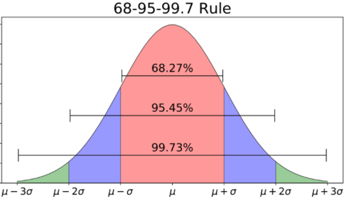
Figure 10.1: 68-95-99 rule of normal distribution
Suppose we take a sample of 397 professor salaries in order to estimate the average salary of all professors at the university. From our sample, we calculate a mean of 113706 dollars and a standard deviation of 30289 dollars. Figure 10.2 below shows the distribution of this sample of salaries.
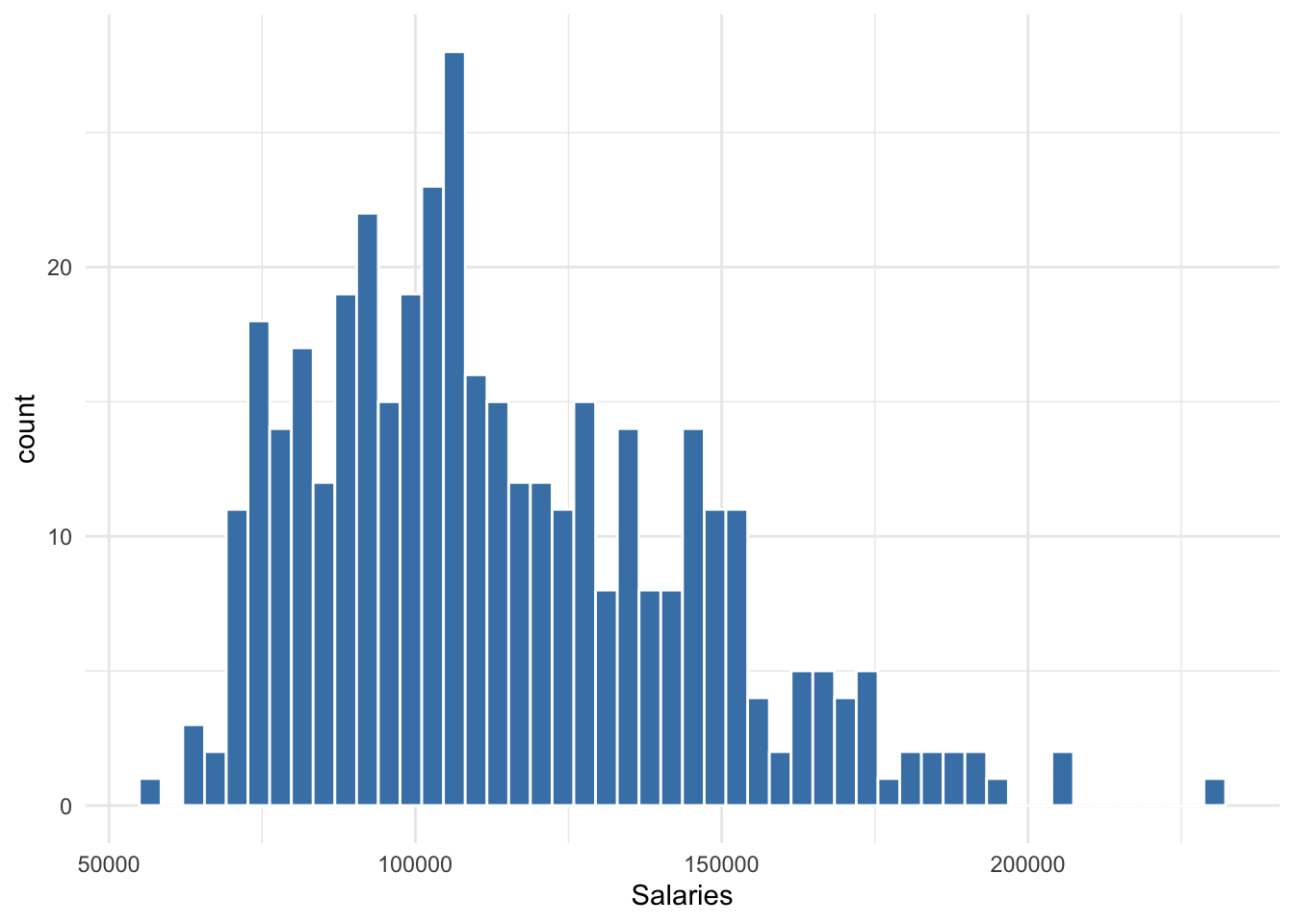
Figure 10.2: Distribution of professor salaries
Note that the distribution of salaries is roughly normal-looking, though it is skewed somewhat to the right. If the distribution of 397 salaries were perfectly normal, then 68% of those salaries fall between 83417 and 143995, 95% percent of the 397 salaries fall within 53128 and 174284, and 99% of the 397 salaries fall within 22839 and 204573. However, since we can observe the entire distribution, we can calculate the range in which 95% of values fall or any percentage of values. The exact 95% range for Figure 10.2 is 70,761 to 181,511.
These ranges are merely descriptions of our sample just like the measures used in Chapter 4. We have not yet made any inference about the salaries of all professors at the university.
Again, it is highly unlikely that the average salary of all professors at the university equals 113706 dollars exactly. Our estimate is a guess of something we do not directly observe. Naturally, we want to know a range in which we can be reasonably confident the average salary of all professors falls. This range is called a confidence interval. However, unlike the distribution of 397 salaries, we only have one estimate from our one sample of salaries. How can we calculate a confidence interval of something we do not observe? To construct a confidence interval, we assume the sampling distribution of the mean of salaries is normal.
10.3 Sampling Distribution
Distributions were covered in Chapter 4. A variable is comprised of multiple values that can be plotted along a number line or axis to form a distribution. This distribution can be described in terms of its center via the mean and its spread via the standard deviation.
A sampling distribution is simply a distribution comprised of multiple estimates, each taken from a separate sample, instead of multiple values, each taken from a separate unit of analysis. Imagine if the distribution in Figure 10.2 were made of 397 averages from 397 samples of salaries. If we have no reason to suspect our estimates are systematically above or below the population mean (i.e. unbiased), then we have a distribution of guesses for the population mean, the center of which should approach the population mean given enough sample estimates. Assuming this sampling distribution is normally distributed, then we can construct an interval in which 95% of the estimates fall as a plausible range in which the unobserved population mean falls.
This tends to be a large theoretical leap for many to make. To reiterate, we have only one sample, not 397. How do we construct a 95% confidence interval off of a sampling distribution we do not have the data to observe? We do so using theory and assumptions. Most importantly, we use the Central Limit Theorem.
10.4 Central Limit Theorem
The Central Limit Theorem may seem like magic more than anything else in statistics, though it is scientifically sound. Given a sufficient sample size, the Central Limit Theorem allows us to assume sampling distributions are normally distributed even though we do not have data to observe the sampling distribution. Without it, we could not construct confidence intervals. Thus, we could not make inferences about a population.
Seeing the Central Limit Theorem work is believing, especially when circumstances are set that would seem to work against it. To do this, let us revisit the distribution of a six-sided die discussed in Chapter 4. With each of the six values having an equal probability of occurring, we know each value has about a 17% chance of occurring. If we were to roll the die some number of times divisible by 6, then all values should occur the same number of times, resulting in a distribution like that depicted in Figure 10.3.
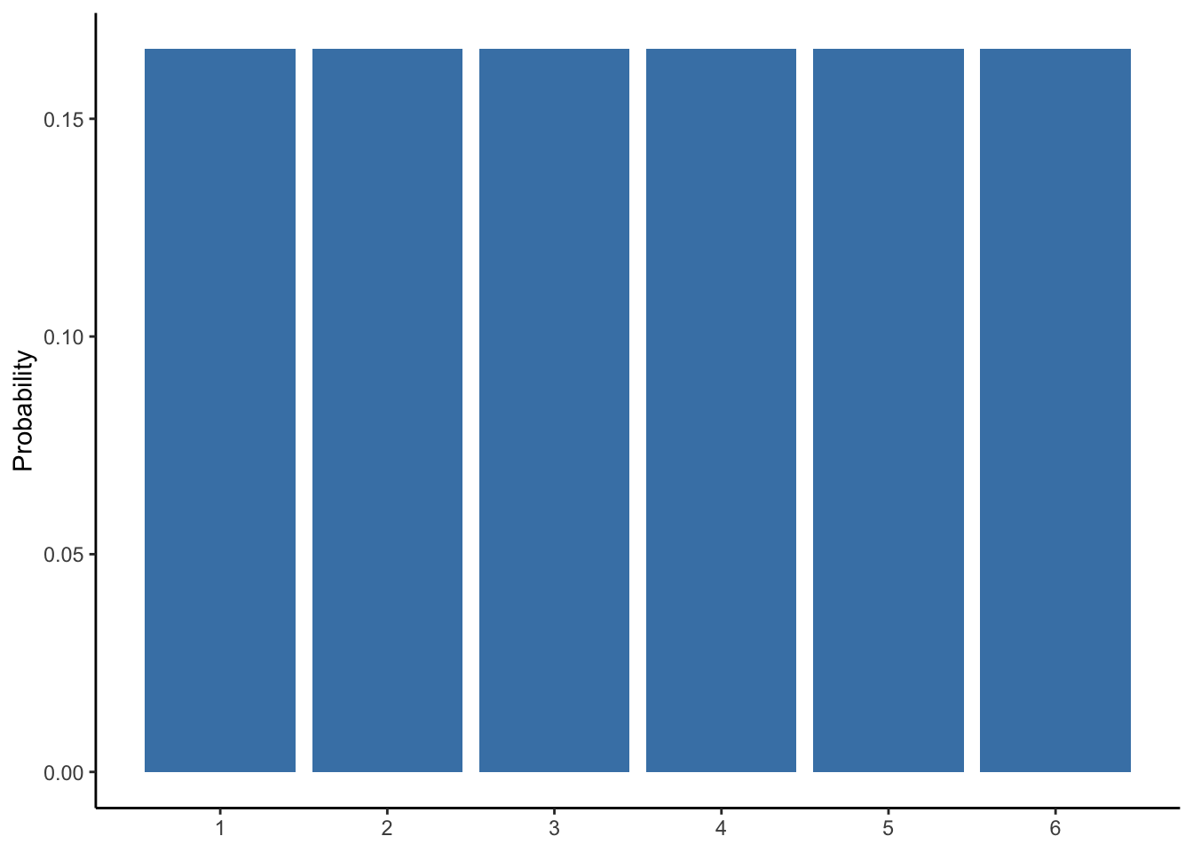
Figure 10.3: Probability distribution of a six-sided die
The distribution in Figure 10.3 is decidedly not normal. Yet, the Central Limit Theorem states that if we took numerous samples from this distribution, each of sufficient sample size, then the sampling distribution will be normal. We typically do not know the distribution of a variable like we do with a six-sided die, thus we do not know where an important measure like the mean is in that distribution. However, if any estimate regarding any variable–no matter the distribution of the variable–is normally distributed, then we do not need to know the distribution of the variable. This is the power and importance of the Central Limit Theorem.
To see how the Central Limit Theorem works, we need a population we can observe but would not be able to in usual circumstances. Suppose we had a population comprised of 10,000 observations. Each observation is the result of rolling a six-sided die. This is obviously a play example for the sake of instruction, but one could imagine the six values of the die to be something more interesting and important, such as levels of education. Table 10.1 below shows a preview of our simulated population.
| ID | education |
|---|---|
| 1 | 2 |
| 2 | 6 |
| 3 | 4 |
| 9998 | 4 |
| 9999 | 6 |
| 10000 | 4 |
Since we have the entire population, we can calculate the population mean, which would typically be a population parameter we cannot calculate. The mean “education level” of this population is 3.518. This is almost exactly equal to the mean we should expect from many rolls of a six-sided die. The distribution of the population’s education is shown in Figure 10.4. The solid red line represents the population mean.
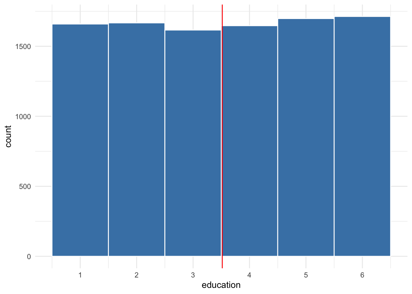
Figure 10.4: Distribution of simulated population
Suppose we were to draw one random sample of 20 from this population. The distribution of this sample is shown in Figure 10.5. The mean of this sample is 3.65, represented by the purple dashed line. The red solid line represents the population mean of 3.518.
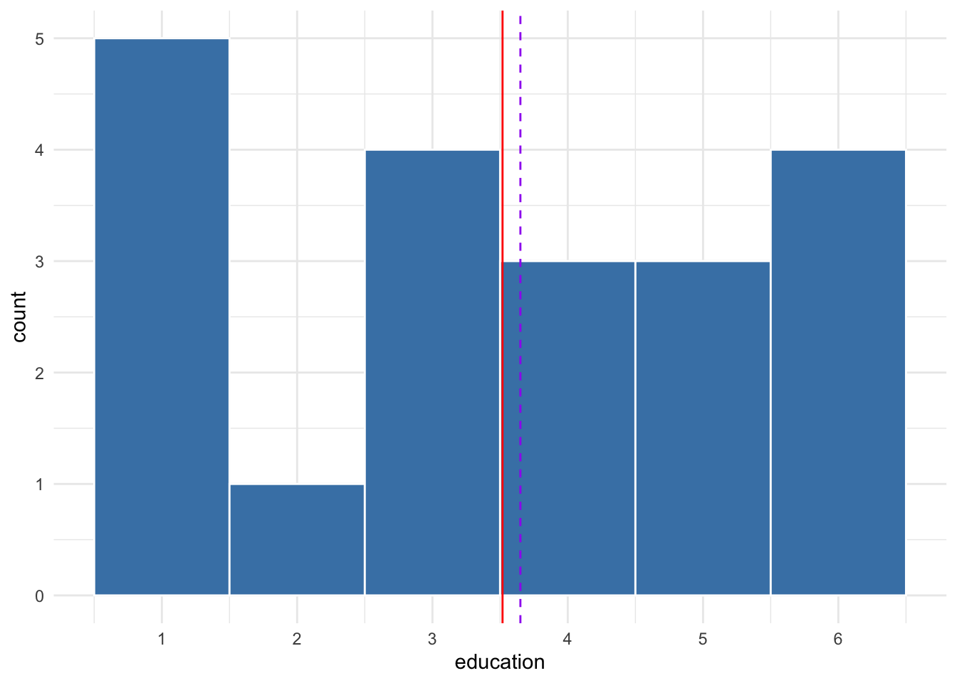
Figure 10.5: Distribution of sample of 20 from simulated population
The sample mean of 3.65 may or may not be a good guess of the population mean of 3.518; such judgments depend on the context of the research question or the decision needing made. Suppose we take a second random sample of 20 from the population, as shown in Figure 10.6. The mean of this second sample is 3.95.
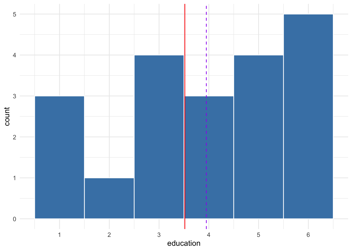
Figure 10.6: Distribution of a second sample of 20 from simulated population
Note that the distribution of the two samples are different and neither are uniform like the population distribution. This is the manifestation of randomness. Each sample gives us a different estimate of the population mean, both of which are too high. Estimates of other samples would fall below the population mean. With enough samples and sample estimates of the mean, we can construct a sampling distribution.
Suppose we take 100 samples of 20 from the population, estimating the mean of each sample to construct a sampling distribution of the mean. This sampling distribution is shown in Figure 10.7. Note that with only 100 samples of only 20 observations each, the sampling distribution roughly resembles the normal distribution. Also, the mean, or center, of the sampling distribution represented by the yellow line is very close to the population mean.
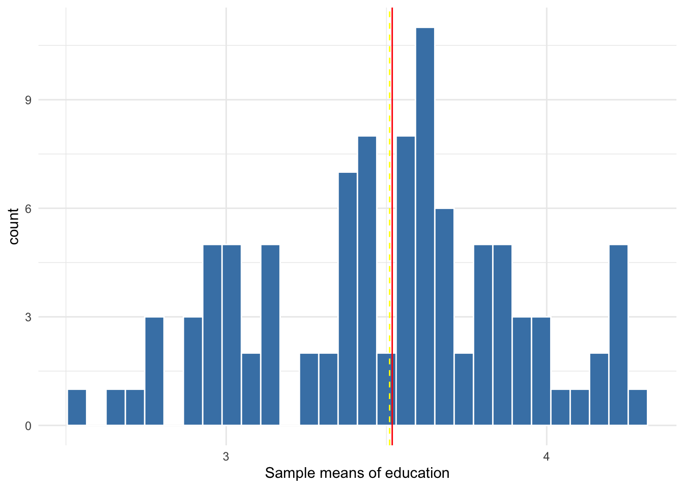
Figure 10.7: Sampling distribution of 100 sample means from samples of size 20
The centering of the sampling distribution at the population mean is due to having an unbiased estimate from random sampling. If our estimate is unbiased, then we expect it to equal the population parameter, on average. This applies to any estimate and its potential bias, including the estimates in regression. If our regression model is unbiased, then our estimate comes from a sampling distribution that centers at the population parameter.
Now let’s take 10,000 samples with a size of 33 observations each, calculating the mean of each sample. The sampling distribution of the 10,000 sample means is shown in Figure 10.8 below. Note that it looks very similar to the normal distribution with a mean equal to 3.157. From a variable that is not normally distributed, we obtain a sampling distribution that is normal. No matter the distribution of the variable, the Central Limit Theorem assures us its sampling distribution will be normal, provided we have a large enough sample.
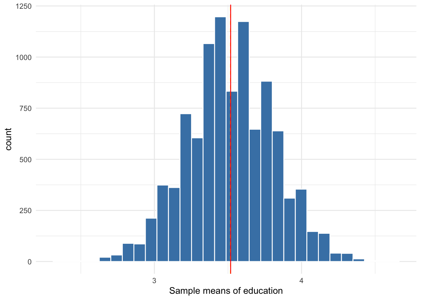
Figure 10.8: Sampling distribution of 10,000 sample means from samples of size 33
In reality, we cannot draw 10,000 samples from the population. If we could, and calculated the mean of the sampling distribution, then we could be extremely confident that we have estimated the population parameter with virtually perfect accuracy. Alas, we have only one sample and no sampling distribution to observe. Though we can safely assume our one estimate comes from a normal sampling distribution that, if there is no bias, is centered at the population mean, we do not know where our sample falls within that distribution. Our one sample could be one with an estimate in or near the left or right tails of the sampling distribution in Figure 10.8. Therefore, we need a range of plausible values for the population parameter. For this range we need to measure the spread of the sampling distribution in terms of its standard deviation.
10.5 Confidence intervals
The standard error is used to construct confidence intervals. The standard error is essentially the same as the standard deviation. It is the name given to the standard deviation of a sampling distribution instead of a variable’s distribution. Now that we can safely assume our sample estimate comes from a normal sampling distribution, and given that we need to account for the randomness of any one sample, we can calculate the range of values within which 95% or 99% of the estimates in the sampling distribution falls. In short, we have returned to applying the 68-95-99 rule, only this time we use it to construct a confidence interval.
The 95% confidence interval for any estimate is 2 standard errors (1.96, technically) below and above the estimate. The 99% confidence interval is about 3 standard errors below and above the estimate. Referring back to the sampling distribution in Figure 10.8, the standard deviation is equal to 0.26. Suppose we drew one sample that gave us an estimate of 4. Suppose the standard error of that estimate happened to equal 0.26. In that case, the 95% confidence interval is approximately 3.48 to 4.52. Since we know the population parameter equals 3.518, we know our confidence interval captures it, which is what we hope to be the case but cannot confirm in typical circumstances.
How do we calculate the standard error to construct the 95% confidence interval or any confidence interval without observing the sampling distribution? Again, theory and assumptions. Throughout this running example, we have been trying to estimate the mean of the population. The standard error (SE) of a sample mean is calculated using the following equation
\[\begin{equation} SE = \frac{s}{\sqrt{n}} \tag{10.1} \end{equation}\]
where \(s\) is the standard deviation of the variable in our sample data and \(n\) is the number of observations in our sample.
Equation (10.1) highlights one of the reasons sample size is a point of interest in analysis. In addition to needing at least 33 observations for the Central Limit Theorem to work reliably, sample size affects the precision of our confidence interval. As \(n\) increases, the denominator in Equation (10.1) increases. Given a standard deviation, greater denominator results in a smaller SE than a lesser denominator. That is, as our sample size increases, the range of our confidence interval decreases.
To demonstrate the effect of sample size on precision, suppose we drew 10,000 samples of size 1,000 instead of 33, as was done for the sampling distribution in Figure 10.8. Figure 10.9 depicts the sampling distribution of this hypothetical scenario. Not that the distribution is virtually identical to normal. Of most importance is the spread of the sampling distribution. The standard deviation of the sampling distribution (or standard error) in Figure 10.8 is 0.26. The standard error of the sampling distribution in Figure 10.9 is equal to 0.05.
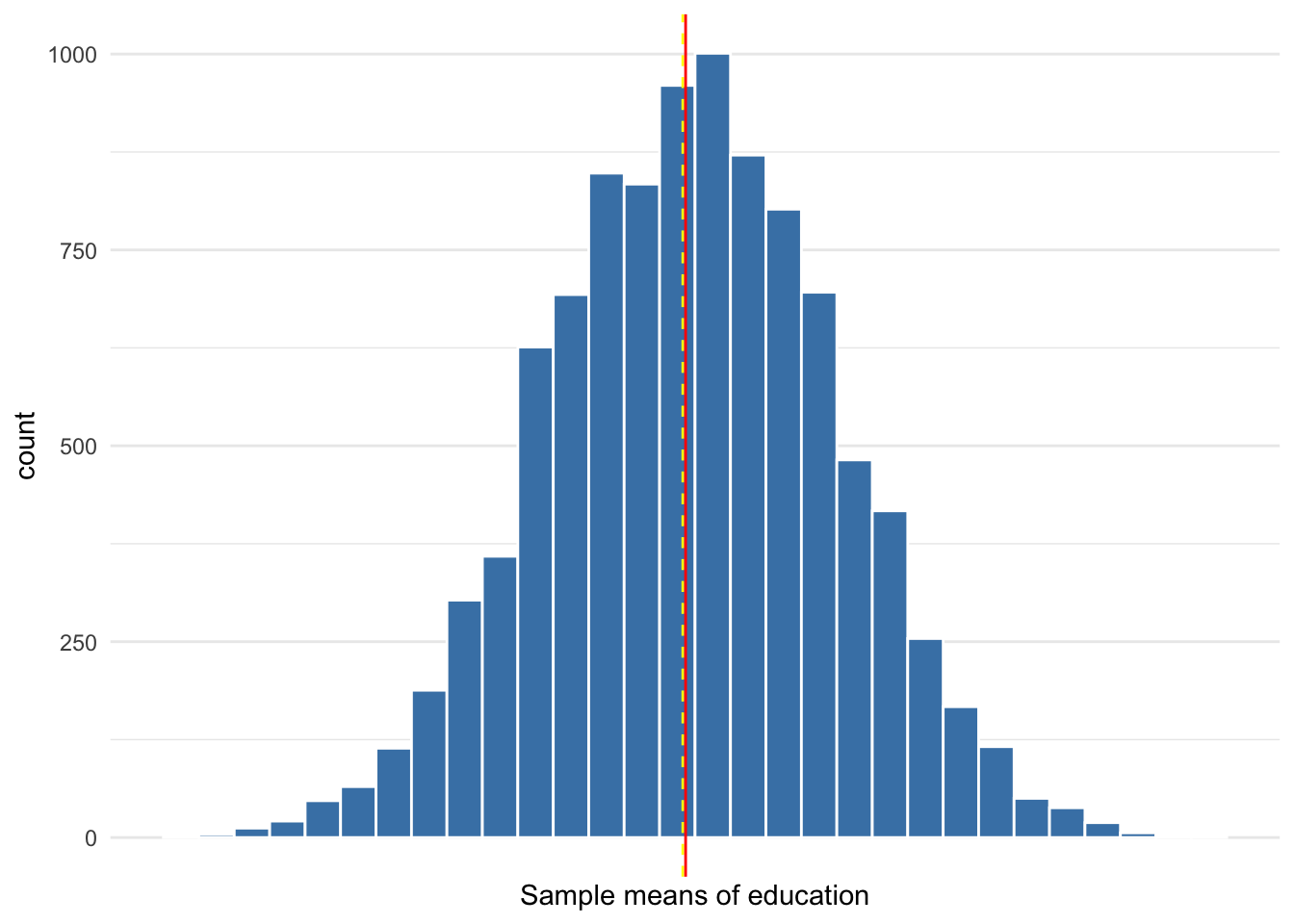
Figure 10.9: Sampling distribution of 10,000 sample means from samples of size 100
From a sample of size 1,000 it is much less likely that we would obtain a sample estimate as far from the parameter of 3.518 as 4. Moreover, whatever our estimate, we can construct a confidence interval with the same level of confidence that will be much smaller. A more precise confidence interval may allow for more confident decision-making.
10.6 Conclusion
Though in reality we obtain only one estimate from one sample, we assume that estimate is one value of a normally distributed sampling distribution that is centered at the population parameter we intended to estimate. Our one sample estimate is highly unlikely to equal the population parameter because of randomness. Therefore, in addition to our specific estimate of the parameter, we construct a range of plausible values that captures that population parameter.
To walk through the full process of estimation using one sample in this simulated data example, one of the 10,000 samples of size 1,000 (sample 379) had a mean education level of 3.552. The standard deviation of education in this sample was 1.53. Given 1,000 observations, then the standard error is equal to
[1] 0.04838285Therefore, assuming a normal sampling distribution and absence of bias, the 95% confidence interval for our estimate of the population mean of education is
[1] 3.45792[1] 3.64608The 95% confidence interval of this particular sample captures the population parameter of 3.518.
A common interpretation of, say, a 95% confidence interval is that our population parameter has a 95% probability of falling within our confidence interval. This is incorrect. A confidence interval either contains the population parameter or it does not. There is no 95% probability to speak of; only 0% or 100%. What a confidence interval conveys is that if we were to draw numerous samples from this population rather than just the one, then we would expect 95% of the confidence intervals constructed from all of our samples to capture the population parameter and 5% of the confidence intervals to fail. Our sample could be one of those 5% of samples for which the confidence intervals fail to capture the population parameter.
One out of 20 samples are expected to fail to capture the population parameter that it was intended to estimate. This is why many have concerns regarding a crisis of replication in science. If only one study is published, and replications of a study are difficult to have published, then we do not know if the one that was published is the anomaly or not.