3 Measurement
“Will he not fancy that the shadows which he formerly saw are truer than the objects which are now shown to him?
—Plato
Once we understand the structure of our data and the types of variables contained within, we need to understand how the data relates to reality before trying to draw conclusions. Variables and their values are measured representations of reality. They are shadows on the allegorical cave wall. We should not assume these shadows are necessarily good representations of reality.
Measurement validity and reliability are the foundations of credible analysis, the components of which are depicted in Figure 3.1 below. Without the two, we have little or no basis to make conclusions from data. As they say, garbage in, garbage out. No amount of fancy statistical techniques can compensate for starting with bad data.
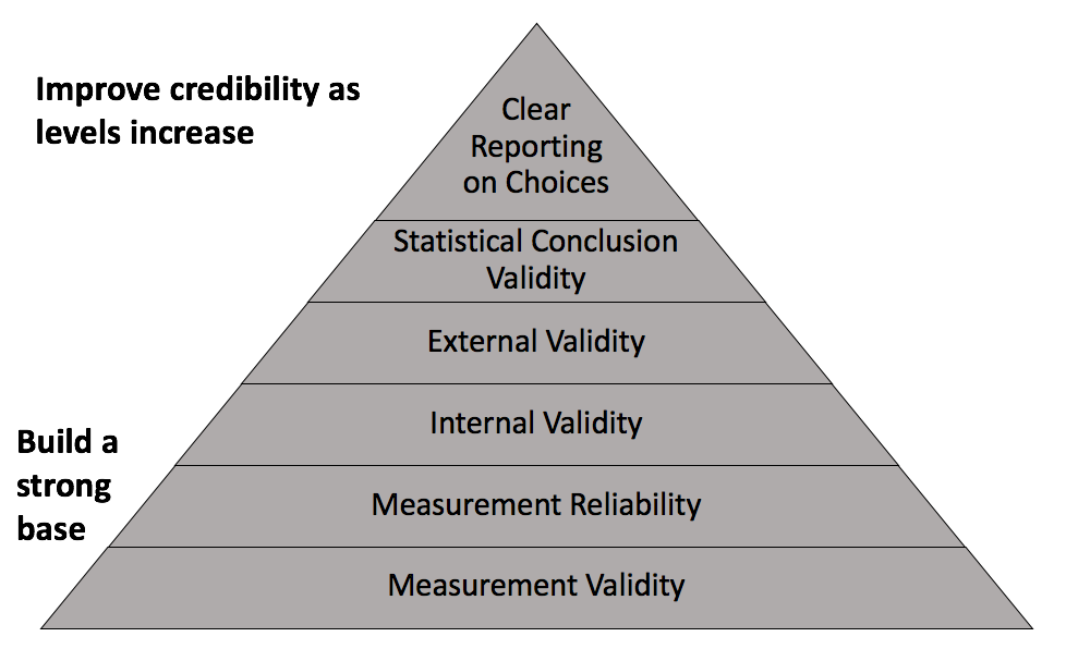
Figure 3.1: Components of credible analysis
3.1 Learning objectives
- Assess the measurement validity of variables
- Assess the measurement reliability of variables
- Explain the difference between accuracy and precision
3.2 Measurement validity
Data do not exist in nature. Someone must set out to observe a phenomenon, measure it, record it, and compile the recorded measures into a dataset. This process involves choices, limitations, and potential flaws. When evaluating the quality of data, the first quality to consider is measurement validity.
Measurement Validity: The extent to which a variable measures what it is intended to measure.
Variables record measures of observed phenomena. Students take a test, resulting in a variable for test scores. Patients’ height and weight are recorded, resulting in a variable for body mass index (BMI). People respond to a survey from the Bureau of Labor Statistics asking whether they are employed or actively looking for a job, resulting in a variable for the unemployment rate. Law enforcement agencies record reported crimes and divide the total by population, resulting in a variable for crime rate.
What do these variables intend to measure? The intent of a variable could be to simply measure the observed phenomenon. A city manager may use a robbery crime rate to understand how many robberies per capita occurred in their city and how this rate has changed over time. Almost all types of crime are systematically under-reported. Therefore, as a variable intended to measure the incidence of robberies, the measurement validity of robbery crime rate is somewhat flawed. Specifically, we could say that robbery crime rates are biased negatively/downwards.
It is often the case that variables intend to measure some less observable concept. Student test scores could be used as a measure of intelligence or academic merit. BMI is used as a measure of healthy weight. The unemployment rate is used as an indicator for economic growth/decline. Crime rates are used to measure public safety. When the values of a variable changes over time, or we observe differences in values across people or places, we might conclude the same is the case for the abstract concept we attach to the variable. Before doing so, we should pause to consider whether the variable actually captures the concept.
One area in public administration where measurement validity is a common concern is performance management. Are test scores a valid measure of school or teacher performance? To what extent should test scores be used to hold low-performers accountable? Is a crime rate a valid measure of police performance? Suppose a city manager observes an increase in the rate of robberies. Should their conclusion be that police performance has declined?
3.3 Measurement reliability
The second quality of measurement to consider is reliability.
Measurement Reliability: The extent to which the measurement process or instrument for a variable generates consistent values.
The measurement reliability of a variable can be with respect to repeated measures over time or across subjects. A student receives a score on their GRE. Provided the student does not study before taking the GRE again, will they receive the same or similar score (referred to as test-retest reliability)? A property value assessor assesses a property. A second assessor assesses the same property. Will they arrive at the same property value (referred to as inter-rater reliability)? Suppose two students are equally knowledgeable on the topics included in the GRE. Will the two students receive the same GRE score? Will two identical properties receive the same property value?
Virtually all measurement processes involve at least some measurement error. Think of measurement error as the spread of recorded values around the true value. The greater the spread/error, the less reliable the measure. Measurement error can be random, such that the spread around the true value is evenly distributed above and below the true value. If measurement error is not random, we should consider whether the factors that cause error are related to the conclusions we want to draw from the data.
Poor measurement reliability threatens our ability to make comparisons over time or across subjects. A city manager may know that the rate of robberies is negatively biased (poor measurement validity) but assume that a change in the rate over time reflects the true change despite both recorded values being less than their true values. However, the true crime rate may not have changed at all if the measurement process generates random fluctuations.
3.3.1 Example
A measure can be valid or invalid and reliable or unreliable, resulting in one of four possible combinations. Let us consider an example where an agency needs to allocate resources to state governments according to the number of persons who are homeless in each state. One method has been to designate a specific day of the year (e.g. January 1st) where government staff and volunteers attempt to conduct a census of homeless people. If the census takers in all states successfully recorded the true count of homeless people, then the resulting dataset would contain a valid and reliable measure.
Suppose the true count of homeless persons for two states is the same. Figure 3.2 depicts this scenario and the three potentially problematic combinations of validity and reliability along a number line.
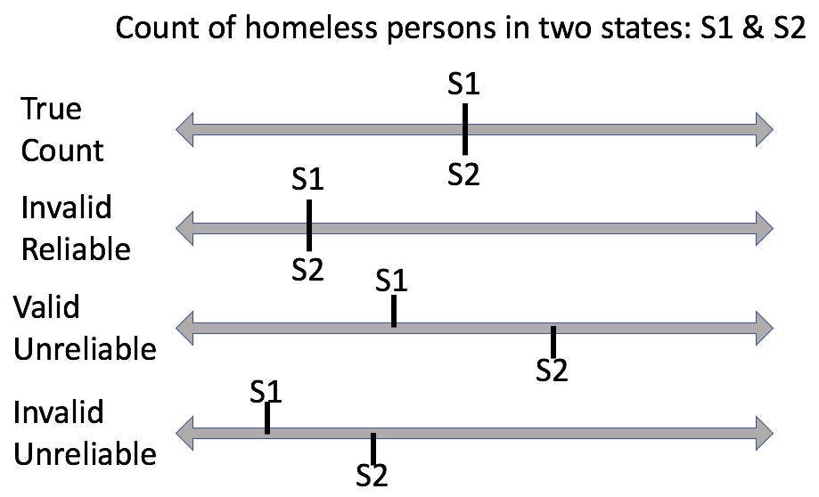
Figure 3.2: Comparing measurement validity and reliability
In the case where a valid and reliable measure is taken, the two states receive equal and appropriate amounts of resources.
The second line in Figure 3.2 depicts a scenario where the number of homeless people are systematically under-counted, but the process generates the same number across the two states. This would be considered in invalid but reliable measure. Resources going to states is less than it should be, but equal states receive equal resources.
The third line in Figure 3.2 depicts what is likely the most confusing combination: a valid and unreliable measure. Homeless people are under-counted in one state and over-counted in the other, but the error is roughly equal. This reflects a case of random measurement error rather than systematic. So long as the spread is not too great, we could consider this a sufficiently valid measure because the recorded values are averaging around the true value. The amount of resources provided is appropriate on average, but the two states receive different amounts.
The fourth line in Figure 3.2 depicts a scenario where an invalid and unreliable measure is taken. Homeless people are systematically under-counted and the error is worse in one state than the other. The two states receive different amounts of resources and the amount of resources provided is systematically less than what it should be.
Taking a count of homeless people on a designated day is known to have issues of measurement validity and reliability. Measurement validity is an issue because it is unlikely that a government can accurately count all of its homeless people. In other words, this measure is negatively biased as depicted in either the second or fourth lines in Figure 3.2.
Even if two states suspiciously had an equal number of homeless people, why might they record undercounts of varying severity? Temperature affects how easily and accurately the number of homeless people can be counted. In a cold state, most homeless people will stay in shelters. In a warm state, homeless people will be scattered and more difficult to count. Differing levels of experience among staff and volunteers is another potential factor.
Keep in mind that no measure is perfect. Our concern should not be so much whether a measure is valid or invalid and reliable or unreliable, but rather the degree to which a measure is invalid and unreliable. When drawing conclusions from a change in values or differences across subjects, take the time to consider the consequences and limitations due to measurement issues.
3.4 Missing data
It is common to encounter missing values in real data. Respondents skip or choose not to answer survey questions, administrators fail to contact respondents, entities that reported data last year may have dissolved or consolidated with another entity this year. Many reasons can lead to missing data. The key is to consider why data are missing and if it should affect your conclusions.
Using the previous example of self-reported income, suppose there are numerous missing values in the responses. Should we assume they are missing at random or that there is some underlying reason or pattern? Perhaps those with no or low income do not wish to report. If we were to dismiss these missing values, and draw conclusions from the non-missing values, we may severely overestimate the income of the target population.
3.4.1 Types of missing data
Missing data come in two varieties:
- Explicit: data that we can see are missing in the data; cells containing a value that denotes missing
- Implicit: data that we would expect to be included based on data structure but are not; no obvious sign of missing
Table 3.1 shows an example of data that are explicitly missing denoted by NA. Missing data is denoted in a variety of ways. For example, instead of NA, the cells could have been left empty, or filled with a period, or some other symbol. If data were obtained from an organization that regularly produces publicly available data, datasets are usually accompanied by a legend that explains what symbols denote missing.
| country | continent | year | lifeExp | pop | gdpPercap |
|---|---|---|---|---|---|
| Argentina | Americas | 2007 | NA | 40301927 | 12779.380 |
| Bolivia | Americas | 2007 | 65.554 | 9119152 | NA |
| Brazil | Americas | 2007 | 72.390 | 190010647 | 9065.801 |
Beware ambiguous missing values. For instance, some survey questions are dependent on previous questions. You do not want to conclude that a value is missing because a respondent chose not to answer when they were never asked the question. Or perhaps a value is missing when it should actually equal 0 or vice versa. If missing data are consequential to your analysis, then you may need to investigate further into how the data were collected or coded in order to eliminate such ambiguity.
Table 3.2 shows an example of implicitly missing data. Argentina is observed in 1997, 2002, and 2007, but Bolivia is observed only in 1997 and 2007. What happened to the 2002 observation for Bolivia? This sort of entry and exit from the dataset is common in panel data where the same units are observed over multiple time periods.
| country | continent | year | lifeExp | pop | gdpPercap |
|---|---|---|---|---|---|
| Argentina | Americas | 1997 | 73.275 | 36203463 | 10967.282 |
| Argentina | Americas | 2002 | 74.340 | 38331121 | 8797.641 |
| Argentina | Americas | 2007 | 75.320 | 40301927 | 12779.380 |
| Bolivia | Americas | 1997 | 62.050 | 7693188 | 3326.143 |
| Bolivia | Americas | 2007 | 65.554 | 9119152 | 3822.137 |
Note that the missing Bolivia observation was easy to spot because the dataset is extremely small. If we were dealing with a large dataset, this would not have been so obvious. A quick way to check whether there may be implicitly missing observations is to check the number of observations in your data. If you are under the impression that your data contains all 50 states for 10 years, then you should have 500 observations. If not, some states or years must be missing.
To learn how to work with missing data in R, proceed to Chapter 18.