16 R Chapter Introduction
This section contains what are referred to as R Chapters, each of which corresponds to a chapter in the previous section. Chapters in the previous section focus on concepts that are applicable regardless of statistical software. R Chapters present those concepts in ways to practically apply them via a short series of exercises using R.
Each R Chapter begins with a list of learning objectives followed by a what you need to set up in terms of packages and data to complete the chapter. Each chapter then guides you through a few exercises that require you to operate R. Periodically, they will ask you to interpret your results and/or connect what you have done to the concept it was meant to help you understand. By the end of each chapter, you will have at least one document to save and upload to eLC. That document will contain code and answers to questions.
Once you upload your R Chapter work to eLC, a document will become available that contains my answers to those same exercises. This is meant to provide almost immediate feedback. You should compare your work to my own, making note of any differences and attempting to make sense of them. Keep in mind that my answers are not necessarily definitive. R Chapters will be incorporated into class discussion when possible, but feel free to ask specific questions about each R Chapter during class.
16.1 What is R and RStudio
R is a programming language for statistical computing. RStudio is a user interface for R. RStudio requires R to be installed on a computer in order to function. Though you need R installed to use RStudio, you never need to launch the actual R program. Instead, you will always use RStudio for assignments in this course.
16.2 Installing R and RStudio
If you intend to install R and RStudio on your computer, follow the instructions below. There are also plenty of videos online that demonstrate downloading R and RStudio if you prefer to have a visual walkthrough.
First, download and install R here.
- Windows user: click on “Download R for Windows”, then click on “base”, then click on “Download R #.#.# for Windows.”
- MacOS user:, click on “Download R for (Mac) OS X.” What you click on next depends on what version of macOS is installed on your Mac and whether your Mac has an Intel chip or Apple chip.
- Under “Latest release,” you will see a link such as “R-4.2.2-arm64.pkg” or “R-4.2.2.pkg” with a description to the right that indicates which versions of macOS it is compatible with, such as macOS 11 (Big Sur) and higher or 10.13 (High Sierra) and higher. If you do not know which version of macOS you are using, click on the apple symbol in the top-left of your screen, then click on “About This Mac.” The resulting window will display your version of macOS.
- If your macOS version is compatible with the latest release, you should download one of the two options under “Latest release.” Note there are different packages to download depending on whether your machine has Apple silicon (M1 and higher) or Intel. Be sure to download the correct package. -If you are using a version of macOS older than 10.13 (High Sierra), scroll down to the header “Binaries for legacy OS X systems” where you can find the link that will work with your version.
- Once you have downloaded R, open the installer file (probably) located in your downloads folder. Follow the prompts to install R, similar to installing any software.
Second, download and install RStudio here.
- Scrolling down this page, you will see “Step 1: Install R,” which you should have already completed. If so, proceed to “Step 2: Install RStudio Desktop”
- The blue box should provide the correct installer based on your operating system. For example, if you are using Windows OS, the blue box should display “Download RStudio Desktop for Windows.” If so, click on the link. If not, scroll down and you will see a list of all installers based on operating system (OS). The second column lists the download link. Click the link that is compatible with your OS.
- Once you have RStudio downloaded, open the installer file (probably) located in your downloads folder. Follow the prompts to install RStudio.
16.3 RStudio orientation
Exercise 1 Launch RStudio
Upon launch, you should see three sections referred to as panes:
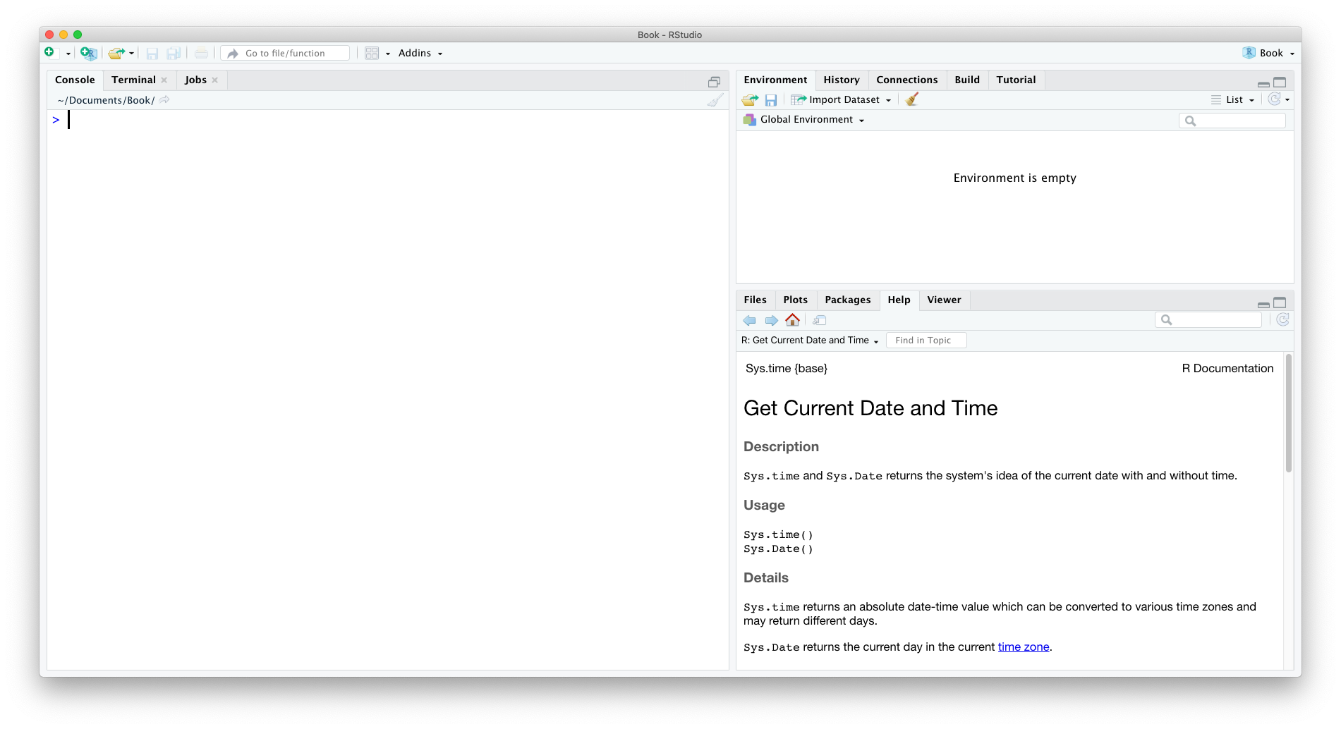
- Console pane (left) is where you can tell R what to do. It also displays the results of commands and any messages, warnings, and errors. You will rarely need to use the console except when installing a package. Only install a package via the console, never as code you would save and (re)run.
- Environment pane (top right) displays all the data in your current R session. A session is the time between launching and closing R.
- Files pane (bottom right) allows you to navigate your files, displays plots, provides a list of installed packages, allows you to search for help, and displays file exports.
You will usually see a fourth pane in the upper-left, with the console in the bottom-left, while working in RStudio – the source editor pane.
Exercise 2 Start a new R Markdown file. You have two
options to do so: 1) See that plus sign (+) icon with a piece of paper
in the very top left of RStudio? Click on that and you will see a list
of options. In this course, we will always use R Markdown documents.
Select R Markdown. 2) In the RStudio menu bar at the top of your screen,
go to File -> New File -> R Markdown. Either way, a
dialog box will appear. You do not need to do anything other than click
OK. A new pane should appear with some default content in
it. This is the pane where you will tell R what to do 99% of the
time because it allows you to write code that you can save.
16.3.1 R Markdown
An R Markdown document allows you to fluidly combine prose that you would write for a report and R code that produces the tables and graphs you wish to incorporate. It can do much more than this, as outlined by this brief video. In this course, we will use R Markdown for R Labs and Problem Sets in addition to these R Chapters.
An R Markdown file consists of two parts:
- YAML Header. The YAML is at the top of your R Markdown file beginning and ending with three dash marks. The YAML sets the global parameters for the document and how it exports. Below is the YAML you may see in your current R Markdown document.
- Body: where you write prose and code. Your current R Markdown document likely opened with some content already in the body. Feel free to read this content, as it is informative.
Exercise 3 In the YAML, change the title to “R Chapter 16”.
Exercise 4 Click on the Knit button at
the top of the source editor pane (looks like a ball of yarn with a
needle stuck in it. If a drop down menu appears, click on
Knit to HTML. RStudio will then prompt you to save your
document. Save your R Markdown file, naming it according to the
following convention (yourlastname_rch16). R will start to
process your document and a new window will appear that contains your
export document. You want to take some time to consider how the code and
prose in the R Markdown document relates to the content you see in the
exported html document. You can close this new window once you are
finished viewing it. Feel free to test Knit to Word if your
computer has Microsoft Word installed. Knit to PDF will not
yet work. RStudio saves your R Markdown document every time you
knit.
16.3.2 R Packages
Many tasks in R require you to install R packages that augment its functionality. This is analogous to a smartphone that comes with base programs (e.g. calendar, weather), but others develop third-party applications to augment its functionality. If you wish to those functions, you go to an app store and download it.
Similarly, when you open RStudio, some base packages are already available that allow you to use a variety of functions. Still, we will almost always need to use functions that require third-party packages.
Install Packages
Two important points to remember throughout this course. First, NEVER install a package from within your R Markdown document (top-left pane). Instead, ALWAYS install a package using the console pane (bottom-left). Installing packages is one of the very few instances in which we use the console pane. Second, you only have to install a package once. If you install a package, you do not need to install it again unless you want or need to update it.
To install R packages, we type the following generic code into the console pane (bottom-left).
Where "name_of_package" is replaced with the actual name of the R package we want to install. If we run this code, it accesses R’s “app store” and downloads the package to your computer. Again, you only need to install a R package once. The package is saved on your computer where R can find it.
Remember to include quotes around the name of the R package when installing it.
Exercise 5 We will almost always need to use a
package called tidyverse. In your console
pane (bottom-left) of RStudio, type
install.packages(“tidyverse”), then click
Enter on your keyboard. This will begin the installation.
Be sure to monitor the console pane while tidyverse
installs. RStudio may ask you some Yes/No questions during the
installation. If you receive the following question:
Do you want to install from sources the package which needs compilation?,
respond with typing no and hit Enter. For any other
questions, respond with typing Yes then click
Enter.
You can install multiple R packages at once. You will need numerous R packages to complete this course. Below is a list of all R packages used in this course except for tidyverse, which you just installed and do not need to install again.
install.packages(c("knitr",
                   "arsenal",
                   "forecast",
                   "fpp2",
                   "lubridate",
                   "readxl",
                   "plm",
                   "broom",
                   "car",
                   "gvlma",
                   "gapminder",
                   "Ecdat",
                   "carData",
                   "openintro",
                   "fivethirtyeight",
                   "moderndive",
                   "DAAG",
                   "Stat2Data",
                   "data.table",
                   "rmarkdown",
                   "tinytex",
                   "DiagrammeR",
                   "jtools",
                   "blogdown",
                   "stargazer"))
Complete the following exercise to download all of the packages needed for the course.
Exercise 6 In your console pane
(bottom-left) of RStudio, copy-and-paste the above code, then click
Enter. This will begin the installation. Again, RStudio may
ask you some Yes/No questions during the installation. If you receive
the following question:
Do you want to install from sources the package which needs compilation?,
respond with typing no and hit Enter. For any other
questions, respond with typing Yes then click
Enter.
Load Packages
When an application is installed on your phone, you still have to launch it (i.e. click on it) to use it. The same goes for using a R package. Each time you launch RStudio, you need to load the package(s) that contain the functions you plan to use. Closing RStudio is like shutting off your phone. When you open your phone, an application isn’t running in the background unless you previously launched it.
Therefore, you should load needed R packages each time you open RStudio. And because you want your code to work each time you or someone else tries to run it, you should include this in your R Markdown document that you save. This is different than installing a package, which you should do in the console, not the saved document.
Remember, you have to load a package every time you restart RStudio. Therefore, type the code that loads a package in the R Markdown document that you save.
The following generic code is loads a package.
Do not use quotes around the name of the R package when loading it. Quotes are only needed to install, not load.
Exercise 7 Near the top of your document, you should
see a code chunk named setup containing the code
knitr::opts_chunk$set(echo = TRUE). Start a new line inside
of this code chunk. Type library(tidyverse) on the new
line. Next, run this code chunk either by clicking on the little
sideways arrow at the right of the code chunk, or by using the keyboard
shortcut Cmd+Enter on Mac or Ctrl+Enter or
Window+Enter on PC. This shortcut only executes the line of
code on which your cursor (the blinking vertical line) is. The console
pane (bottom-left) will provide information about the loading.
Remember, you must load a package before using any functions included in that package or else you will receive the following error message,
Error: could not find function. I will tell you what packages are needed to complete all assignments, but remember that you need to install and load the package to use it.
16.4 Save and Upload
Save your document once more either by knitting again or like any other software – clicking on the floppy disk icon in the menu at the top or using the menu bar File -> Save As. Then upload your .Rmd document to eLC. Once you upload, answers will become available on the Welcome module of eLC.
16.5 Additional Resources
There are many resources that provide orientations to R. Below are two that I consider particularly helpful and accessible.
- Chapters 1-3 of Getting Used to R, RStudio, and R Markdown
- BasicBasics of RYouWithMe by R-Ladies Sydney