6 Simple and Multiple Regression
“You can lead a horse to water but you can’t make him enter regional distribution codes in data field 97 to facilitate regression analysis on the back end.”
—John Cleese
6.1 Learning objectives
- Identify and explain the components of a population or sample regression model
- Explain the difference between a deterministic equation of a line and a statistical, probabilistic equation of a line
- Given regression results, provide the predicted change in the outcome given a change in the explanatory variable(s)
- Given regression results, provide the predicted value of the outcome given a value of the explanatory variable(s)
- Explain what the error term in a regression model represents
- Interpret measures of fit in a regression model and explain their relative strengths and weaknesses
6.2 Basic idea
The basic idea of regression is really quite simple. Regression calculates a line through a scatter plot of two variables so that we can summarize how much our variable on the y axis changes given a change in the variable on our x variable. Or, we can use a given value for our x variable to predict a value for our y variable. That’s all it is–a line drawn to represent the association between two variables.
We all learned the equation for a line back in middle school, which probably looked something like the following:
\[\begin{equation} y = mx + b \tag{6.1} \end{equation}\]
where \(m\) is the slope of the line and \(b\) is the y-intercept. If we know the slope and intercept for a line, then, given a value for \(x\), we can compute \(y\). Given a change in \(x\), we can compute a change in \(y\) by multiplying the change in \(x\) by \(m\).
Consider the following equation for an arbitrary line:
\[y = 5x + 10\]
Here are some questions we can now answer:
- How much does \(y\) change if \(x\) increases by 1? Answer: 5
- How much does \(y\) change if \(x\) increases by 10? Answer: 50
- How much does \(y\) change if \(x\) decreases by 10? Answer: -50
- What does \(y\) equal if \(x\) equals 2? Answer: 20
- What would \(y\) equal if \(x\) were 0? Answer: 10
If you understand how to answer the above questions, then you can interpret regression results for any given context because
interpreting regression results involves either predicting the change in \(y\) given a change in \(x\) or predicting the value of \(y\) given a value of \(x\).
What is different in regression is how the equation of the line is presented because there are population and sample versions of the relationship between \(x\) and \(y\). Also, regression is not a deterministic mathematical equation like the one above. Because we generally use regression to measure relationships between social phenomena, there is inherent uncertainty in the line we calculate. This adds some complexity beyond solving a line’s equation, but the process of running a regression to estimate the slope and intercept of a line to then predict changes or values of an outcome is fundamentally the same as the simple equation above.
6.3 Simple linear regression
Equation (6.2) presents the population regression model.
\[\begin{equation} y=\beta_0+\beta_1x+\epsilon \tag{6.2} \end{equation}\]
Only one element differs between Equations (6.1) and (6.2). That is the symbol at the end, which is the Greek letter epsilon and is used to denote the aforementioned uncertainty of predicting real-world, particularly social, phenomena.
The y-intercept denoted as \(b\) in Equation (6.1) has been moved to the front of the right-hand side in Equation (6.2) and is denoted by \(\beta_0\) (pronounced beta-naught). The slope denoted as \(m\) in Equation (6.1) is now denoted as \(\beta_1\) in Equation (6.2). These beta, \(\beta\), symbols are simply the standard notation for population parameters in a statistical model and are used to signal that we intend to estimate these parameters using regression.
Recall that a parameter is a statistical measure of a population. In most cases, our research questions concern a population so large or inaccessible such that we do not observe all members. Instead, we take a sample of the population. From this sample, we calculate sample statistics, or estimates of the parameters and use methods of inference to decide if these estimates are valid guesses of the parameter (more on this in Chapters 10 - 12).
Equation (6.3) presents the sample regression equation.
\[\begin{equation} \hat{y}=b_0+b_1x \tag{6.3} \end{equation}\]
The carrot symbol atop our outcome variable \(y\) is called a hat, and so the term on the left-hand side is commonly referred to as “y-hat.” This is used to denote the fact that any value we calculate from Equation (6.3) is an estimate of what has been or will be observed. Similarly, the \(b\) symbols are the sample estimate analogs of the \(\beta\) population parameters in Equation (6.2).
Equation (6.3) is the equation we use to interpret our regression results in the same way as was demonstrated using the mathematical equation of a line. Again, the only difference is that we are dealing with a statistical or probabilistic equation of a line–the outcome we calculate is a prediction based on observed data.
6.3.1 Using regression
Let’s pause the theory to consider a simple example using data for U.S. counties. Table 6.1 provides a preview of the data
| name | state | fed_spend | poverty | homeownership | income |
|---|---|---|---|---|---|
| Traverse County | Minnesota | 20.038786 | 9.3 | 80.3 | 41287 |
| Wabash County | Illinois | 7.422533 | 13.0 | 80.1 | 46026 |
| Pike County | Mississippi | 9.091897 | 25.3 | 72.9 | 30779 |
| Greenbrier County | West Virginia | 9.029030 | 19.4 | 75.0 | 33732 |
| Ray County | Missouri | 5.795480 | 9.4 | 78.7 | 53343 |
| Hamilton County | Tennessee | 10.188056 | 14.7 | 65.5 | 45408 |
| Ballard County | Kentucky | 11.907989 | 13.0 | 83.3 | 41228 |
where fed_spending is the amount of federal funds allocated to the county per capita, poverty is the percent of the population in poverty, homeownership is the percent of the population that owns a home, and income is per capita income. There are 3,123 observations in this dataset.
Suppose we wanted to examine the association between federal spending and poverty for U.S. counties such that poverty explains federal spending. After all, a substantial portion of federal dollars are dedicated to assist those in poverty. First, we might visualize the relationship between the two variables.
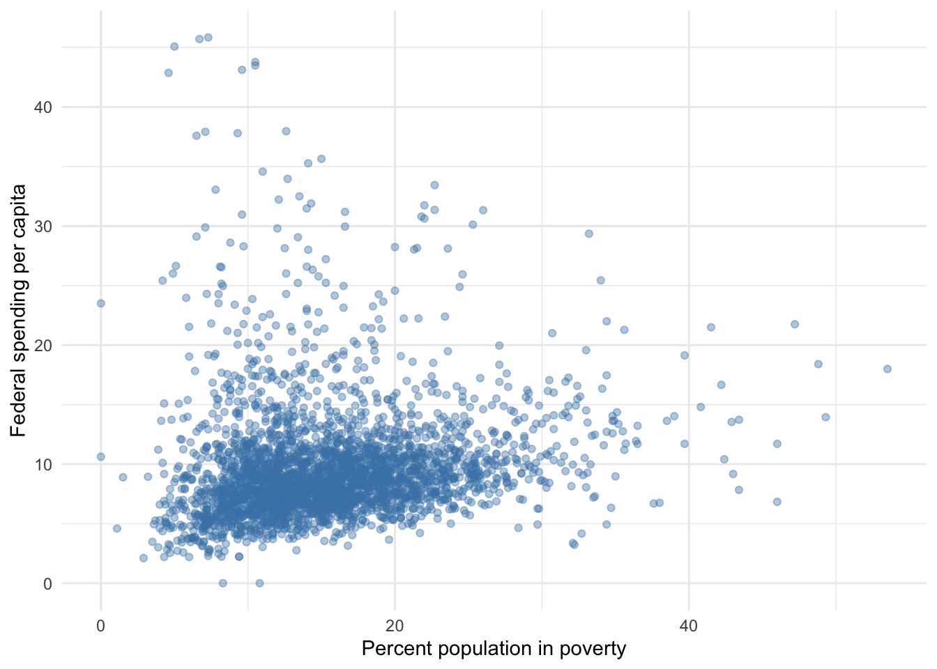
Figure 6.1: Federal spending and poverty among U.S. counties
If we were to trace a line through these points, it would clearly slope upward. This suggests to us that as the percent of the population of a county in poverty increases, the amount of federal spending it receives increases. But by how much? That is what regression estimates for us.
Equation (6.4) represents the relationship between federal spending and poverty using a simple linear regression population model. Note that we have chosen to model the two variables such that poverty explains or predicts federal spending. This aligns with the choice to plot poverty on the x axis and federal spending on the y axis in Figure 6.1. This is a critical choice in every regression and one that computers still need humans to help with (more on that later).
\[\begin{equation} FedSpend = \beta_0+\beta_1Poverty + \epsilon \tag{6.4} \end{equation}\]
We are going to use observed values of poverty and federal spending to estimate \(\beta_0\) and \(\beta_1\). Then, once we have those estimates, we can provide succinct answers regarding how federal spending tends to change given a change in poverty or a predicted level of federal spending given a particular level of poverty in a county.
The \(\epsilon\) represents all the other factors that explain or predict federal spending that are not in our model. If our world were such that the points in 6.1 literally formed a straight line, we would not need an \(\epsilon\), but this is never the case with interesting questions of complex phenomena. This may or may not be a problem for whatever story we intend to tell about the the relationship between poverty and federal spending.
Running the regression as represented in Equation (6.4) produces Table 6.2 of results.
| term | estimate | std_error | statistic | p_value | lower_ci | upper_ci |
|---|---|---|---|---|---|---|
| intercept | 7.950 | 0.219 | 36.294 | 0 | 7.520 | 8.379 |
| poverty | 0.108 | 0.013 | 8.265 | 0 | 0.082 | 0.134 |
With the exception of Chapter 9, this section on regression focuses on understanding the methods used to generate the values in the estimate column immediately to the right of the variable names as well as how to interpret and apply these values to any question. The remaining columns in the above table pertain to inference and will be covered in the section on inference.
The values in the estimate column are commonly referred to as coefficients, which were first mentioned in Chapter 4. Regression coefficients measure the direction and magnitude of association between an explanatory variable and an outcome variable.
Now that we have our results, we can plug them into our sample regression equation like so
\[\begin{equation} \hat{FedSpend}=7.95+0.108 \times Poverty \tag{6.5} \end{equation}\]
and we are back to the first section of this chapter. Note that we replaced the intercept, \(\beta_0\), with our estimate of the intercept, \(b_0=7.95\) and replaced the marginal effect of poverty on federal spending, \(\beta_1\), with our estimate of the marginal effect, \(b_1=0.108\).
The intercept of a regression does not always have a practical use. The intercept represents the predicted value of the outcome when the explanatory variable \(x\) equals 0.
Note in Figure 6.1 that it appears only two counties in the US have a poverty rate of 0, so it is not a very applicable scenario. Still, our regression model suggests that federal spending per capita is predicted to equal $7.95 when the poverty is 0.
We are usually more interested in the estimates corresponding to our explanatory variable(s). The estimates for our explanatory variables represent their marginal effect on the outcome. That is, as \(x\) changes one unit, \(y\) changes by \(b\) units.
There is a standard template for reporting the marginal effect or estimate of a explanatory variable in regression. It goes as follows:
On average, a one [unit] increase in \(x\) [is associated with] a \(b\) [unit] [increase/decrease] in \(y\).
A couple points about the above template:
- We replace [unit] with the actual units of the \(x\) variable (e.g. dollar, percentage point)
- We replace \(x\) with what \(x\) is
- We can replace [is associated with] with any combination of words to express the relationship (e.g. causes, results in, tends to, etc.)
- We replace \(b\) with the value of the estimate from our regression results
- We replace [unit] with the actual units of the \(y\) variable, and
- We replace \(y\) with what \(y\) is
Applying this template to our example, we can write the following:
On average, as the percent of the population in poverty increases by 1 percentage point, federal spending per capita tends to increase approximately 11 cents.
The marginal effect of poverty on federal spending is 11 cents. A couple points about the above interpretation:
- We always qualify with “on average” because that is exactly what regression does. Drawing a line through a scatter plot results in points above and below that line. Will every instance of a one percentage point increase in poverty result in an increase of 11 cents in federal spending? No. Sometimes it is more, and other times it is less. The line drawn by regression traces how \(y\) responds to \(x\) on average.
- The standard change in \(x\) to use when reporting results is one unit. Poverty is in units of percent. Therefore, a one-unit change in a variable measured in percentages is one percentage point (e.g. 10% to 11%).
6.3.2 Predicted change
Any hypothetical change in the explanatory variable can be used to predict the corresponding change in outcome. To do so, we only use the part of the regression equation that includes the explanatory variable that is changing:
\[\begin{equation} \Delta \hat{y}=b_1x \tag{6.6} \end{equation}\]
where \(\Delta\) denotes change. We replace \(b_1\) with our estimate and \(x\) with the magnitude of the hypothetical change. This gives us the predicted change in \(\hat{y}\) given the particular change in \(x\).
Applying this to our example, what is the predicted change in federal spending per capita given a 10 percentage point increase in the poverty rate?
\[0.108 \times 10 = 1.08\]
Federal spending per capita is predicted to increase by an average of $1.08 given a 10 point increase in county poverty rate.
6.3.3 Predicted value
Any hypothetical value of the explanatory variable can be used to predict the corresponding value of outcome. To do so, we use the full regression equation.
For example, if we expected a county’s poverty rate to be 30%, then we could report a predicted level like so.
\[7.95 + 0.108 \times 30 = 11.19\]
Given a poverty rate of 30%, federal spending per capita is predicted to be $11.19, on average.
6.3.4 Visualizing predicted change and value
Figure 6.2 visualizes the regression line from our running example. Note that when poverty equals 0, the regression line appears to intersect the y-axis of federal spending just below $10, which we know is exactly $7.95 from our regression results in Table 6.2. Also, we know the slope of this line is 0.108.
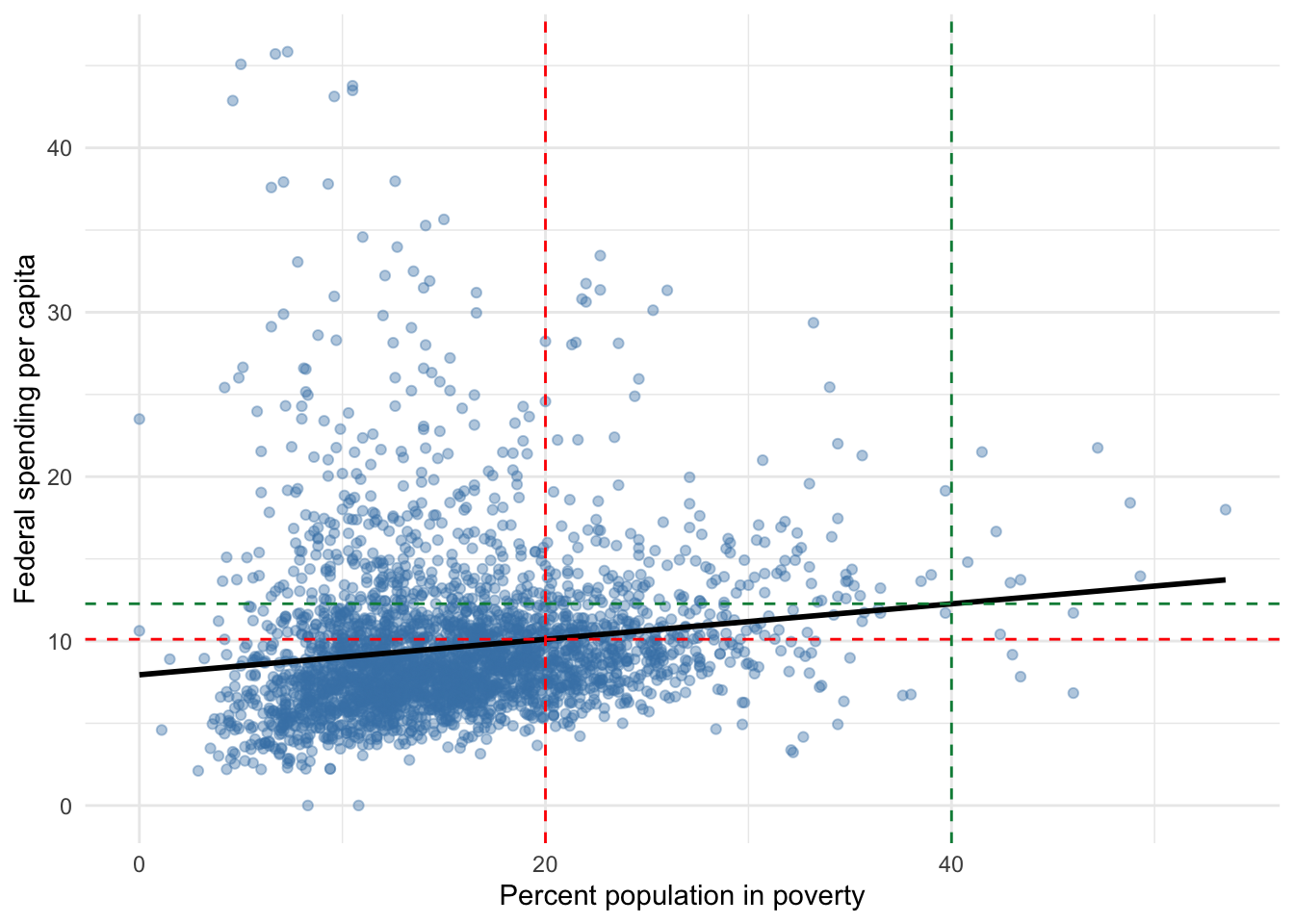
Figure 6.2: Federal spending and poverty among U.S. counties
The dashed red and green lines visualize how our regression line (or the equation from which it is drawn) is used to predict change in the outcome and/or the value of the outcome. It may not be clear why we do not use the intercept when predicting change. The vertical red line represents a poverty rate of 20% and the vertical green line represents a poverty rate of 40%. If we were to ask what the predicted change in federal spending per capita is if the poverty rate were to increase by 20 percentage points, the answer is the vertical distance between the horizontal red and green lines. In other words, if we were to move along the regression line from 20 to 40, how much distance will we cover along the y-axis? This only involves the slope of the line, not where the regression line intersects the y-axis. The vertical distance between the horizontal red and green lines is
[1] 2.16or $2.16. Federal spending per capita is predicted to increase $2.16 given a 20 percentage point increase in poverty. Because this is a linear regression line, a 20 percentage point increase starting from any poverty rate would predict the same change because \(0.108 \times 20\) always equals 2.16.
Hopefully, it is clear why we use the entire regression equation to predict the value of the outcome given the value of the explanatory variable. In Figure 6.2, the predicted value of federal spending per capita at poverty rates of 20% and 40% is where the horizontal red and green lines intersect the y-axis, respectively. Precisely, predicted federal spending per capita at 20% poverty is
[1] 10.11and predicted federal spending per capita at 40% poverty is
[1] 12.27Note that the difference between the predicted values at 20% and 40% is
[1] 2.16which is a roundabout way of getting the predicted change in federal spending given a 20 point increase in poverty and demonstrates why we do not need to incorporate the intercept when predicting change. When predicting the value of federal spending, not incorporating the intercept would be as if the regression line intersects the y-axis at 0, which is clearly not the case here. Without the intercept, our answer for predicted federal spending per capita at 20% and 40% poverty would be
[1] 2.16and
[1] 4.32each of which underestimates predicted federal spending by exactly the intercept
[1] 7.95[1] 7.956.3.5 The error term
Back to theory. We need to address this \(\epsilon\) that is present in the population regression model but disappears in the sample regression model and results. What gives?
The \(\epsilon\) term is commonly referred to as the error term or, for those who don’t like to insinuate some error was made in the regression, statistical noise. I prefer error term if for no other reason than to remind us to consider the myriad of errors we may be making in our regression model.
As mentioned, the error term represents the inherent uncertainty of modeling an outcome based on a necessarily finite number of explanatory factors. Other factors affect our outcome. As a matter of principle, failure to account for all other factors that affect our outcome does not prohibit our attempt to estimate the effect of a variable we care about on the outcome.
Could we account for multiple factors (i.e. multiple regression)? Absolutely. Can we control for everything that affects our outcome? Definitely not if you subscribe to chaos theory or philosopher David Hume’s thoughts on causality. Even if not so extreme as to say our world is too complex to ever make decisions concerning one variable’s effect on another, the plausibility for us to collect data on every relevant factor is highly unlikely.
So, where did the error term go? It never really left; it simply is not used when calculating the predicted outcome based on our regression results. Like our \(\beta\) terms, the error term is a population parameter. However, unlike the \(\beta\)s, we do not have observed data that corresponds to the error term’s estimation. In fact, the concept of the error term exists on the basis that we do not observe it. Therefore, it is necessarily excluded when we predict an outcome based on observed data, all the while we are careful to remind readers that the numbers we report are estimates subject to error and everything we report is based on an average.
If the error term never left, where is it? Its sample analog exists as the difference between our estimated regression line and the observed data. Figure 6.3 below highlights each residual in our running example.
Warning: Using `size` aesthetic for lines was deprecated in ggplot2 3.4.0.
ℹ Please use `linewidth` instead.
This warning is displayed once every 8 hours.
Call `lifecycle::last_lifecycle_warnings()` to see where this warning
was generated.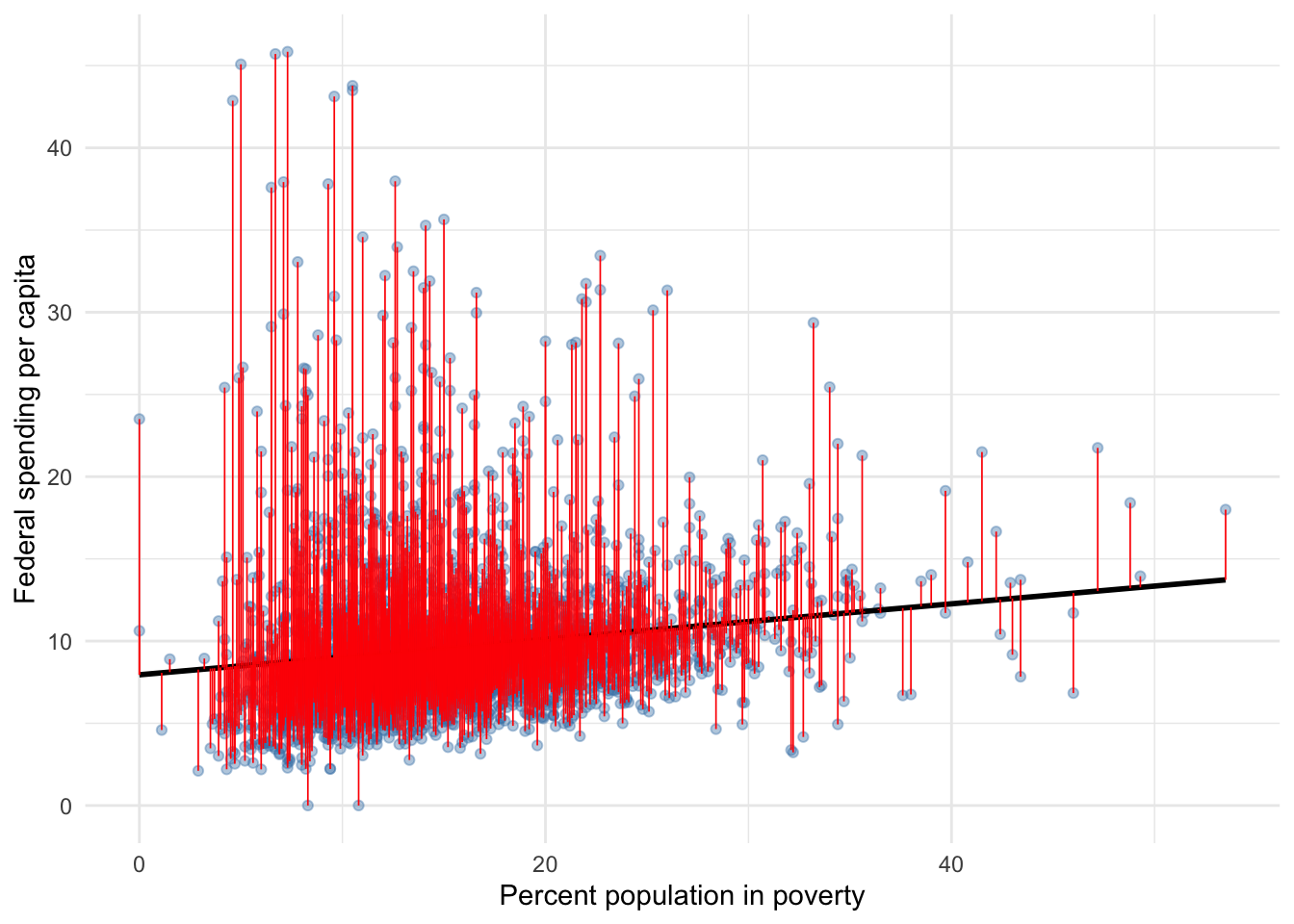
Figure 6.3: Federal spending and poverty among U.S. counties
Surely, it is apparent that our regression line does not intersect all points perfectly; many points lie above or below our line. The vertical distance of any line between a plot point and the regression line in Figure 6.3 is the values of a particular residual. In this example, our residuals are in units of dollars of federal spending per capita.
Table 6.3 quantifies the error/residual for select observations.
| ID | fed_spend | poverty | fed_spend_hat | residual |
|---|---|---|---|---|
| 1961 | 7.592 | 16.9 | 9.773 | -2.181 |
| 2440 | 10.188 | 17.1 | 9.795 | 0.393 |
| 1738 | 15.784 | 8.8 | 8.899 | 6.885 |
| 2641 | 23.503 | 0.0 | 7.950 | 15.554 |
| 1471 | 8.152 | 25.0 | 10.647 | -2.495 |
| 1362 | 7.649 | 14.0 | 9.460 | -1.811 |
| 2792 | 7.933 | 13.5 | 9.406 | -1.474 |
Our regression model uses observed values of poverty and federal spending to estimate the parameters of the regression line, which produced Equation (6.5). We can then plug the observed values of poverty into the equation to compute a predicted level of federal spending, represented by fed_spend_hat. For example, for observation 1,961 in our data, actual observed federal spending per capita was $7.59. However, given that this county’s poverty rate was 16.9, our regression model predicts federal spending per capita to be
[1] 9.7752as we can see in the fed_spend_hat column ( \(\hat{y}\) ).The right-most column of Table 6.3 shows the difference between predicted federal spending and observed federal spending. Again, this difference is called the residual. Our regression over-estimates federal spending for this county by $2.18. Thus, the residual for this county is -2.18 because the observed outcome is 2.18 less than the estimated outcome.
The residual is represented mathematically by Equation (6.7)
\[\begin{equation} e = y - \hat{y} \tag{6.7} \end{equation}\]
where \(e\) is the sample analog of \(\epsilon\). This is simply the equation behind the process of differencing the observed and predicted values of our outcome just described.
6.3.6 Goodness of fit
Armed with an understanding of error and its sample analog, the residual, we can now consider goodness-of-fit. We must accept there will be error in our regression, but that does not mean we do not seek to minimize that error as much as possible.
Assessing fit
Table 6.4 provides a standard set of three goodness-of-fit measures often used to assess regression.
| r_squared | adj_r_squared | rmse | nobs |
|---|---|---|---|
| 0.021 | 0.021 | 4.654482 | 3123 |
The first column titled r_squared refers to the measure \(R^2\), also known as the coefficient of determination defined in 4. The \(R^2\) measures the strength of association between a set of one or more explanatory variables and an outcome variable. Specifically, it quantifies the percent of total variation in the outcome explained by our regression model. In this case, our regression using poverty explains 2.1% of the total variation in federal spending.
The column titled rmse refers to root mean squared error (RMSE). The RMSE quantifies the typical deviation of the observed data points from the regression line and is particularly useful when predicting a value for our outcome. For example, if after predicting that a county with 30% poverty will receive 11.25 dollars of federal spending per capita, someone asks us how far off that prediction is likely to be, the RMSE suggests our prediction will tend to be off by plus or minus 4.65 dollars.
Regression involves choices. We choose which variables to use to explain or predict an outcome and how to model their effect on the outcome. This menu of choices will become increasingly evident as we build our regression toolbox. As we make choices, competing regression models emerge from which we must choose the one we prefer to report for decision-making.
The \(R^2\) and RMSE provide us the basis for choosing our preferred model. In general, we prefer the model with a higher \(R^2\) and/or a lower RMSE. In virtually all cases, these two measures will agree with each other; the model with the higher \(R^2\) will also have the lower RMSE.
For a more thorough treatment of fit that is unessential but potentially helpful, check out 6.3.6.
6.4 Multiple regression
Of course, we are not limited to using only one variable to explain or predict an outcome. In fact, it is rather uncommon to use only one variable, but simple linear regression is useful for introducing the method of regression. Now, we can consider more realistic modeling method where we use multiple explanatory variables in our regression, which is aptly named multiple regression.
Equation (6.8) provides the population model for multiple regression
\[\begin{equation} y=\beta_0+\beta_1x_1+\beta_2x_2+\cdots+\beta_kx_k+\epsilon \tag{6.8} \end{equation}\]
The only difference in this equation compared to Equation (6.2) is the inclusion of multiple explanatory variables. Each explanatory is numbered and has a corresponding parameter \(\beta\) representing the marginal effect it has on the outcome. In theory, we can add however many explanatory variables we deem worth including, represented by the arbitrary \(k\).
Equation (6.9) presents the sample equation for multiple regression.
\[\begin{equation} \hat{y}=b_0+b_1x_1+b_2x_2+\cdots +b_kx_k \tag{6.9} \end{equation}\]
Again, nothing is different from before except for more explanatory variables and sample estimates of the parameters.
6.4.1 Using multiple regression
Let’s return to our example of federal spending per capita in U.S. counties. Previously, we used only the percent of the population in poverty to explain or predict federal spending per capita. Let’s add the percent of the population that owns a home and per capita income to our model. Thus, our model can be written as such
\[\begin{equation} FedSpend = \beta_0 + \beta_1Poverty + \beta_2HomeOwn + \beta_3Income + \epsilon \tag{6.10} \end{equation}\]
which generates the following results
| term | estimate | std_error | statistic | p_value | lower_ci | upper_ci |
|---|---|---|---|---|---|---|
| intercept | 23.519 | 1.333 | 17.645 | 0.000 | 20.905 | 26.132 |
| poverty | -0.056 | 0.021 | -2.674 | 0.008 | -0.097 | -0.015 |
| homeownership | -0.126 | 0.012 | -10.736 | 0.000 | -0.149 | -0.103 |
| income | 0.000 | 0.000 | -7.723 | 0.000 | 0.000 | 0.000 |
and the following goodness-of-fit measures
| r_squared | adj_r_squared | rmse | nobs |
|---|---|---|---|
| 0.064 | 0.063 | 4.55216 | 3123 |
Now we can discuss what is different with multiple regression. First, note that our coefficient or estimate for poverty has changed from 0.108 to -0.056. Why the change? Because we are controlling for other factors. Part of the marginal effect we reported poverty had on federal spending in our simple regression model was misattributed from the marginal effects of homeownership and/or income on federal spending.
This is a key feature of multiple regression:
it estimates the marginal effect of a variable on an outcome, holding all other explanatory variables equal to their respective means. In other words, if we were omnipotent beings who could take each county in our data and set homeownership and income to the mean of homeownership and income according to the observed data, then pull some lever that makes poverty change and nothing else, the estimate for poverty in our multiple regression reports how much each percentage point in poverty changes federal spending.
This is how we isolate the effect of one variable on an outcome despite knowing other variables simultaneously affect our outcome.
The interpretation of multiple regression estimates is essentially the same as simple regression. In our example, we can interpret the homeownership estimate like so:
On average, our results indicate that a one percentage point increase in the percent of the population that owns a home is associated with a decrease in federal spending per capita of approximately 13 cents, holding other factors constant.
The part in bold is to point out the small difference between the two interpretations. Here, we are simply reminding a reader that we have controlled for other factors that presumably we have already explained, and our estimate for poverty accounts for those factors by holding them constant. Other common word choices for this part of the interpretation include “all else equal” or its Latin translation “ceteris paribus.”
Again, we can answer any sort of question relevant to our original research question concerning the predicted change or level of federal spending by plugging in the numbers to our regression equation.
\[\begin{equation} \hat{FedSpend} = 23.52 - 0.056 \times Poverty - 0.13 \times HomeOwn + 0 \times Income \end{equation}\]
If we wanted to predict the change in federal spending given an 3 percentage point increase in poverty and a decline in home ownership of 4 percentage points, the our answer would be
[1] 0.336dollars per capita (on average and all else equal, of course). If we wanted to predict the level of federal spending per capita for a county with 12% poverty, a 80% home ownership rate, and $31,000 income per capita, then we would predict
[1] 12.767dollars per capita.
Not so fast! This example provides a good opportunity to consider another aspect of the units our variables are in. Per capita income is in dollars. This means the estimate for income represents the effect of a one dollar change in per capita income on federal spending per capita. That’s a very small change that we would expect to have a very small effect on federal spending. This effect is so small that statistical software may round to 0. But what if we changed the units of income to thousands of dollars per capita instead of dollars per capita? Then we get the following results.
| term | estimate | std_error | statistic | p_value | lower_ci | upper_ci |
|---|---|---|---|---|---|---|
| intercept | 23.519 | 1.333 | 17.645 | 0.000 | 20.905 | 26.132 |
| poverty | -0.056 | 0.021 | -2.674 | 0.008 | -0.097 | -0.015 |
| homeownership | -0.126 | 0.012 | -10.736 | 0.000 | -0.149 | -0.103 |
| income_1000 | -0.086 | 0.011 | -7.723 | 0.000 | -0.108 | -0.064 |
Now we see the effect of a one thousand dollar change in per capita income on federal spending per capita. Note that the estimates for poverty and homeownership are the same. Therefore, the predicted level of federal spending for our county is actually
[1] 10.101dollars per capita. Note that because income is in units of 1,000, a county with an income of 31,000 per capita must be rescaled to 31 in the regression equation.
6.4.2 Fit and adjusted R squared
In addition to doing a better job isolating the marginal effect of one variable on an outcome, including additional explanatory variables can reduce the error in our regression, thus achieve more accurate and/or precise predictions of the outcome.
We can assess this improvement in fit by comparing the results in Table 6.6 to those in Table 6.4. We have gone from an RMSE of 4.65 dollars to an RMSE 4.55 dollars. This means our predictions from the multiple regression model tend to be off by 10 cents fewer than the predictions of our simple regression model.
The previous discussion on fit conspicuously skipped over the column titled adj_r_square because adjusted-\(R^2\) applies when comparing two or more models with a different number of explanatory variables.
One caveat to using \(R^2\) to choose a preferred model is that it mechanically increases as the number of explanatory variables increases whether those additional variables improve the extent to which our regression explains the total variation in the outcome or not. Therefore, it is unfair to compare a model with one explanatory variable to a model with more than one explanatory variable.
The adjusted-\(R^2\) accounts for this unfairness by applying a penalty to each additional explanatory variable. We can fairly compare models with different numbers of explanatory variables using their respective adjusted-\(R^2\).
In our example, the adjusted-\(R^2\) for the simple regression model equals 0.021, while the multiple regression model has an adjusted-\(R^2\) of 0.063. Therefore, the multiple regression model is the statistically superior model.
When reporting how much variation in the outcome our preferred model explains, we should still use its \(R^2\). Our preferred, multiple regression model explains 6.4% of total variation in federal spending. Adding home ownership and income has more than doubled the explanatory power of our model of federal spending.
6.4.3 Explanatory penalty
Each explanatory variable we add to our regression model imposes a type of penalty on our results. Basically, for each explanatory variable included, we lose an observation in our data (not literally). This will be discussed further in the section on inference, but we need at least 33 observations to make valid inferences about a population based on sample estimates. If we had, say 50 observations in a dataset, and wanted to run a regression with 25 explanatory variables, then it is as though our regression model is based on only 25 observations (50 observations - 25 variables = 25 degrees of freedom). We will obtain results from such a model, but we probably should not use those results to make inferences.
In case you were wondering why not simply add all the variables we can to a model rather than carefully consider which variables to include and exclude in a model, this penalty is one of the primary reasons. Fewer degrees of freedom jeopardizes our ability to make valid inference. It can also reduce the precision of our predictions.
One of our goals with regression should be to maximize the explanatory or predictive power of our regression model at minimal cost (i.e. excluding superfluous variables).
Choosing good regression models is where subject matter expertise plays a crucial role. Experience and knowledge within the context of the research question informs our choices. Statistics is the method by which we apply our expertise to data to make evidence-based decisions.
6.5 Key terms and concepts
- Line concepts
- y-intercept
- slope
- change in y versus value of y
- Regression model components
- outcome/dependent/response variable
- independent/explanatory variable
- error term/statistical noise
- residual
- population parameter
- sample coefficients/estimates
- Goodness of fit
- R-squared
- Adjusted R-squared
- root mean squared error (RMSE)
- Controlling for other factors in multiple regression