15 Panel Analysis
“The more things change, the more they are the same.”
—Jean-Baptiste Alphonse Karr
15.1 Panel data
Recall from Chapter 2 that panel data measures the same units over multiple time periods. Table 15.1 below provides an example of panel data. Panels for geographic or political areas such as counties, school or voting districts, states, and countries are common and easy to obtain. Due to privacy protections and challenges of following people over time, panels of individual people are somewhat more difficult to obtain but are quite common.
| country | continent | year | lifeExp | pop | gdpPercap |
|---|---|---|---|---|---|
| Argentina | Americas | 1997 | 73.275 | 36203463 | 10967.282 |
| Argentina | Americas | 2002 | 74.340 | 38331121 | 8797.641 |
| Argentina | Americas | 2007 | 75.320 | 40301927 | 12779.380 |
| Bolivia | Americas | 1997 | 62.050 | 7693188 | 3326.143 |
| Bolivia | Americas | 2002 | 63.883 | 8445134 | 3413.263 |
| Bolivia | Americas | 2007 | 65.554 | 9119152 | 3822.137 |
Cross-sectional data is like having a single picture for each unit among multiple units. We use variation across those units with respect to some variable (e.g. income, unemployment rates) to explain or predict outcomes of interest. Time series is like having a video of one subject, following that subject over multiple time periods. We use variation over time to explain or predict outcomes of interest for that subject. Panel data is like having videos for multiple subjects. Therefore, we have variation across units and over time to use for explaining or predicting outcomes of interest.
15.2 Fixed effects
The additional information contained within panel data affords us a wide array of new analytic techniques that go far beyond the scope of this book. There is one technique or model, however, that is probably the most common and very easy to use: the fixed effects model.
Recall the standard multiple regression model shown below. This model is slightly different from what you have seen before because it uses indexing to indicate that we have panel data. This indexing is done with the i and t subscripts, which represent subject and time, respectively. It is simply used to convey that we have multiple subjects i over multiple time periods t.
\[\begin{equation} y_{it}=\beta_0+\beta_1x_{1it}+\beta_2x_{2it}+\cdots+\beta_kx_{kit}+\epsilon_{it} \tag{15.1} \end{equation}\]
A fixed effects model is a slightly modified version of Equation (15.1) that represents an important conceptual leap. Recall that the \(\epsilon_{it}\) term represents all the factors that are associated with or affect the outcome \(y_{it}\) that we cannot include in our model for various reasons. This error term is inevitable and not a problem as long as there are no factors that also affect any of our explanatory variables. Otherwise, we have omitted variable bias in our model and may not be able to use our results.
In most cases, someone can probably think of an omitted variable that is related to one or more of the explanatory variables. In other words, it is really difficult to convincingly guard against claims of omitted variable bias. However, having panel data allows us to guard against an important source of potential OVB by using a fixed effects model. Using a fixed effects model allows us to control for all of the omitted factors that do not change over time.
The fixed effects model is represented in Equation (15.2) below. Note the new term (the Greek letter alpha) immediately to the right of the equal sign has replaced the usual y-intercept, \(\beta_0\), term. Also, note the index for this new term only includes i. Because our data contains a time series for each subject i, we can model a unique y-intercept for each subject. The unique y-intercepts represent all of the stuff that makes the subjects inherently different from each other and do not change over time, or at do not meaningfully change over the time span of our data.
\[\begin{equation} y_{it}=\alpha_{i}+\beta_1x_{1it}+\beta_2x_{2it}+\cdots+\beta_kx_{kit}+\epsilon_{it} \tag{15.2} \end{equation}\]
The fixed effect model is essentially identical to controlling for a categorical variable like we saw in Chapter 7. Recall the graph below where we controlled for the region each state is in when modeling the relationship between miles driven and traffic fatalities. We controlled for region not because we thought being in the West literally causes drivers to have more fatal accidents, but rather because regions might capture unobserved geographic or infrastructure characteristics that affect traffic fatalities.
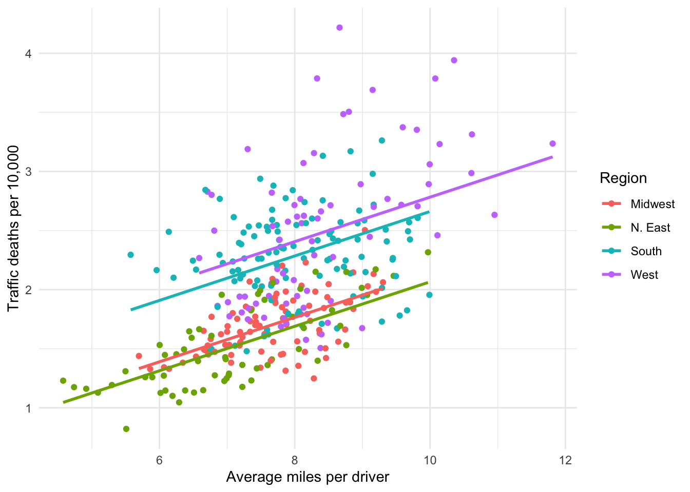
Figure 15.1: Parallel slopes for 4 groups
The fixed effect model takes this idea a little further, controlling for the unobserved characteristics of each unit–the state in this case–rather than some aggregated level like region. This produces a separate regression line for each unit, as seen in Figure 15.2. For unobserved reasons, states seem to have inherent differences with respect to miles driven and fatalities. Note how flat the common regression slope is for all of the states compared to the slope of the regression without fixed effects in Figure 15.3. Ignoring the inherent differences between states leads to the conclusion that distance driven has a larger effect on the fatality rate than what the data actually suggests once we control for those differences. This is the primary reason for using a fixed effects model.
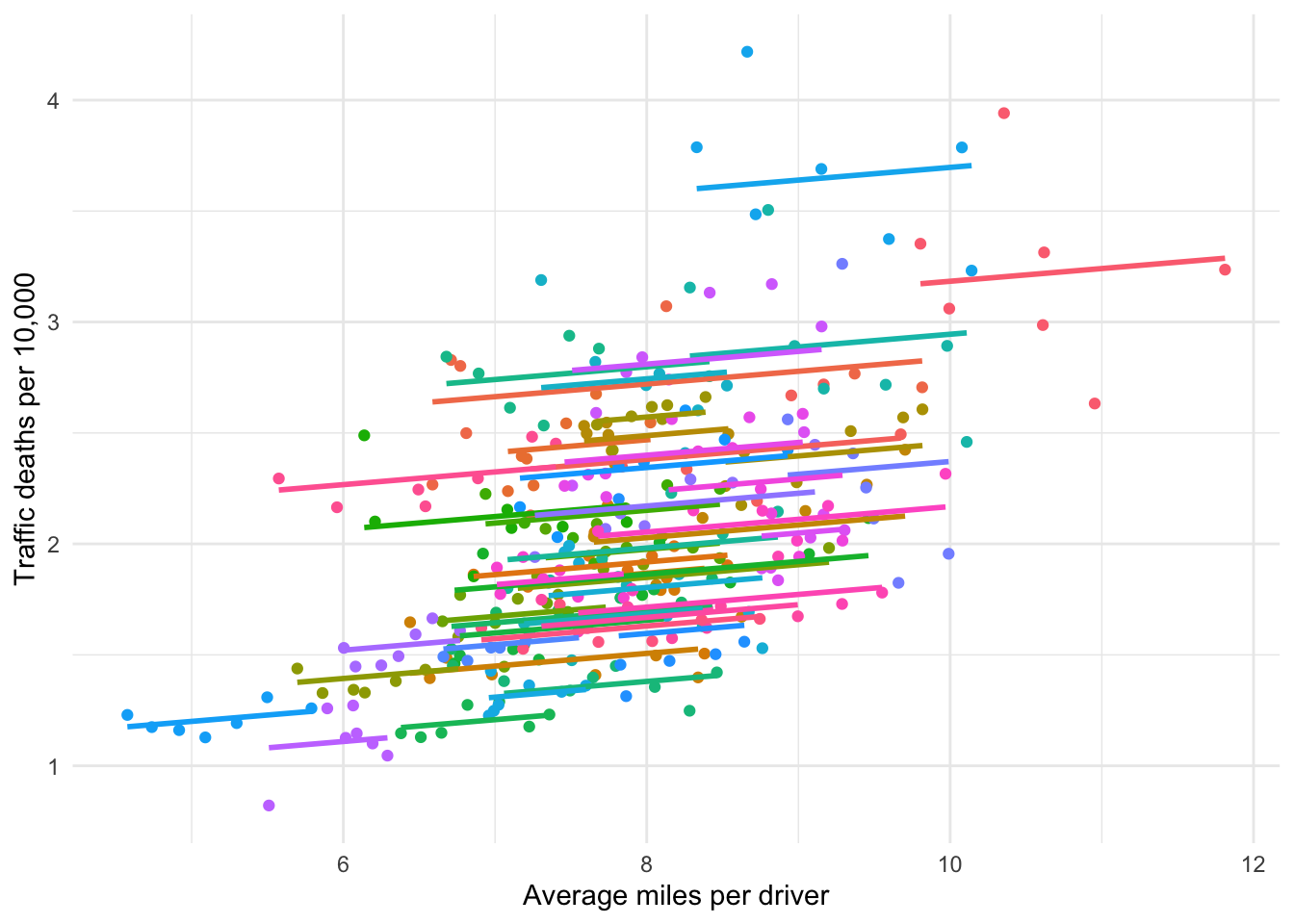
Figure 15.2: Visualizing fixed effects
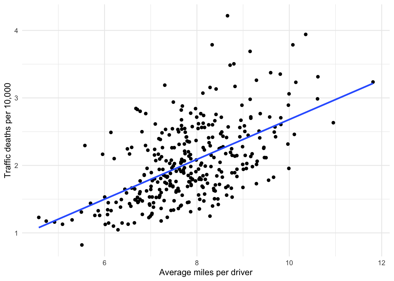
Figure 15.3: Ignoring fixed effects
There is one trade-off of using fixed effects that casual users should be aware of: using a fixed effect absorbs all constant variables. Variables that tend not to change over time such as race, sex, geography, membership to some higher-level unit (e.g. employee within an agency or union) all collapse into the fixed effect. This means that we will not obtain an estimate for these variables in a fixed effects model because they are also fixed. If we really care about getting an estimate from a time-invariant variable, then we cannot use a fixed effects model.
For example, recall the regression results we obtained in Chapter 7 for the following parallel slopes model.
\[\begin{equation} mrall = \beta_0 + \beta_1vmiles + \beta_2region + \epsilon \tag{15.3} \end{equation}\]
| term | estimate | std_error | statistic | p_value | lower_ci | upper_ci |
|---|---|---|---|---|---|---|
| intercept | 0.260 | 0.167 | 1.553 | 0.121 | -0.069 | 0.589 |
| vmiles | 0.188 | 0.021 | 8.895 | 0.000 | 0.147 | 0.230 |
| region: N. East | -0.076 | 0.065 | -1.166 | 0.245 | -0.204 | 0.052 |
| region: South | 0.519 | 0.056 | 9.283 | 0.000 | 0.409 | 0.630 |
| region: West | 0.641 | 0.062 | 10.264 | 0.000 | 0.518 | 0.763 |
We got estimates for three of the regions, providing us average differences in the traffic fatality rate relative to the fourth excluded region.
Running a fixed effects model for Equation (15.3) generates the following results. Note the absence of a single intercept because there is a separate intercept for each state that typically is not included in a table. More importantly, there is no estimate for the regions because a state’s region is absorbed by the state’s fixed effect.
We are left with an estimate for the only variable in our model that differs across time within each state: vmiles. The estimate is statistically significant at the standard 5% significance level and is substantially less than the estimate in the model ignoring fixed effects. Here, as the average miles driven per driver within a state increases by 1 mile, the fatality rate increases by 0.057 deaths, all else equal.
| term | estimate | std.error | statistic | p.value |
|---|---|---|---|---|
| vmiles | 0.057 | 0.019 | 2.956 | 0.003 |