C Goodness of Fit

The discussion below is an extension of Chapter 6’s coverage of goodness-of-fit.

Regression draws the best line through a set of data points of two or more variables. The best line in this case is the line with a slope and y-intercept that minimizes the sum of squared residual between the set of data points and said line. The procedure used to achieve such a line is called ordinary least squares (OLS). The type of regression covered in this book is sometimes referred to as OLS regression.

Recall that the variance of a variable is the sum of squared deviations from the mean, as depicted in Equation (4.2). This should sound familiar. Instead of deviations from the mean, fitting the best line in regression concerns the deviations from the regression line, which by definition are the residuals. As with variance, we square the deviations (i.e. residuals) for the data used to estimate the regression line, then we add these squared deviations together to obtain the sum of squared residual (SSR). Equation (C.1) shows this process mathematically.

\[\begin{equation} SSR=\sum _{i=1}^{n}(y_{i}-\hat{y})^2= (y_{1}-\hat{y})^2+(y_{2}-\hat{y})^2+\cdots +(y_{n}-\hat{y})^2 \tag{C.1} \end{equation}\]

SSR quantifies the error in our regression and is what regression minimizes when predicting an outcome given the explanatory variables we have chosen to include.

The SSR also provides us what we need to compute the root mean squared error (RMSE). Recall that in order to compute the variance and standard deviation of a variable in Equations (4.2) and (4.3), respectively, we divide the sum of squared deviations by the number of observations (or \(n-1\)) then take the square root. The SSR is a sum of squared deviations. The deviations in this case represent error. If we divide SSR by the number of observations, we now have the mean of the sum of squared error. Then, if we take the square root, we have the root mean squared error. Note that this is the same process used to obtain the standard deviation. Thus, the RMSE is the regression version of a standard deviation. Just as the standard deviation tells us the average deviation from the mean, the RMSE tells us the average deviation from the regression line, or the average error in our regression.

We can also quantify the extent to which our regression explains the outcome. To do so, we need a benchmark against which to compare the reduction in error achieved by our regression. This benchmark is simply the average value of the outcome. If we had no explanatory variables to predict an outcome, the mean provides the typical value of the outcome. If we had to draw a random observation from a variable’s distribution, the mean is our best guess of what that observation’s value would be if we have no explanatory variables.

Figure C.1 adds a reference line of average federal spending to our scatter plot. Note that because average federal spending is a constant number, it does not change as poverty changes; the red line has no slope. Also, note that the red line does slightly worse fitting the data, particularly toward the left and right extremes of poverty. Compared to the red line representing the mean, the data appear to be more centered around our regression line. As a result, our regression line has less error than the mean.

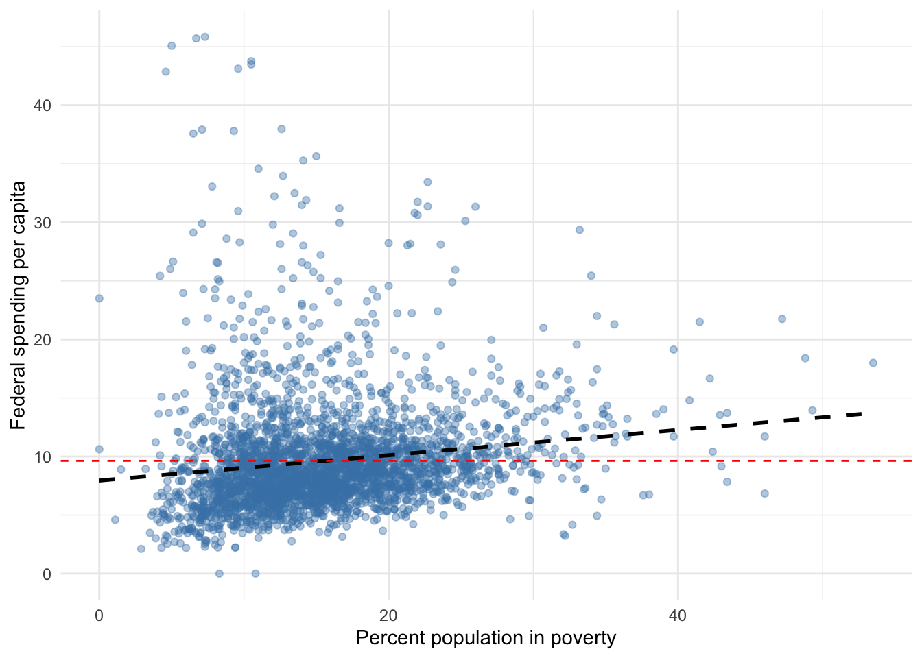
Figure C.1: Federal spending and poverty among U.S. counties

The mean of the outcome is our benchmark for assessing how much the explanatory variables included in our regression model explains the total variation in the outcome. The difference, if any, between the values our regression predicts, \(\hat{y_i}\), and the mean, \(\bar{y}\), serves as the basis for quantifying the extent to which our regression model explains the total variation in the outcome. Just like with the SSR, we square the difference between each predicted value and the mean, then add them together. The result is called the sum of squared explained (SSE) and is represented mathematically in Equation (C.2).

\[\begin{equation} SSE=\sum _{i=1}^{n}(\hat{y}_{i}-\bar{y})^2= (\hat{y}_{1}-\bar{y})^2+(\hat{y}_{2}-\bar{y})^2+\cdots +(\hat{y}_{n}-\bar{y})^2 \tag{C.2} \end{equation}\]

We now have the sum of squared residuals (SSR) and sum of squared explained (SSE). Together, the SSR and SSE represent the sum of squared total (SST) variation in the outcome \(y\).

\[\begin{equation} SST = SSR + SSE \tag{C.3} \end{equation}\]

Recall that the \(R^2\) measures the percent of total variation in the outcome that is explained by our regression. To calculate any percent we take divide a proportion of the whole divided by the whole (e.g. \(5/10 = 0.5\) or 50%). Thus, to obtain the percent of variation in the outcome explained by our regression, we divide the SSE by SST.

\[\begin{equation} R^2 = {\frac{SSE}{SST}} \tag{C.4} \end{equation}\]

The better you understand the mechanics of simple linear regression, the easier it will be to understand the next section and subsequent chapters on regression models because they are mere extensions of this basic model.