7 Categorical Variables and Interactions
“For how can one know color in perpetual green, and what good is warmth without the cold to give it sweetness?”
—John Steinbeck, Travels with Charley
Chapter 6 introduced regression models that contain only continuous variables. In this chapter, we build our regression toolbox to include models that contain categorical variables. We will cover three models in particular:
- Parallel slopes model: including a categorical explanatory variable
- Interaction model: allowing the slope of the regression line for each level of a categorical variable to differ (i.e. not parallel)
- Linear probability model: including a two-level (binary) categorical outcome
7.1 Learning objectives
- Explain why and how to extend simple or multiple regression models to a parallel slopes model
- Interpret results of a parallel slopes model
- Explain why and how to extend regression models to an interaction model
- Interpret results of an interaction model
- Provide advice on choosing between parallel slopes and interaction model
- Explain why and how to extend regression models to a linear probability model
- Interpret results of a linear probability model
7.2 Parallel slopes model
To introduce the inclusion of categorical variables in regression, the simplest type of categorical variable will be used. The simplest categorical variable is commonly referred to as a dummy variable.
A dummy variable is a two-level or binary categorical variable. It takes on values of either 1 or 0, where 1 corresponds to “yes” or “true” and 0 corresponds to “no” or “false”.
For example, a common way to represent biological sex in data is to use a dummy variable where either male or female is coded as 1 and the other sex is coded as 0 (it remains uncommon to find data that codes gender as non-binary either). The convention is to name such a variable whatever level is coded as 1. For example, a dummy variable coded as 1 for male and 0 for female will often be named “male” in a dataset. A variable coded as 1 to denote a person attained a college degree and 0 to denote they did not might be named something like “college.”
The parallel slopes model using a dummy variable is represented in Equation (7.1).
\[\begin{equation} y = \beta_0 + \beta_1x + \beta_2d + \epsilon \tag{7.1} \end{equation}\]
where \(d\) is simply used to distinguish the variable as a dummy variable whereas \(x\) represents a numerical variable as introduced in Chapter 6. The sample regression equation for the parallel slopes model is represented by Equation (7.2).
\[\begin{equation} \hat{y} = b_0 + b_1x + b_2d \tag{7.2} \end{equation}\]
Knowing that \(d\) can equal only 1 or 0, we can plug these values into Equation (7.2) to understand the logic of the parallel slopes model before considering an example. If \(d=0\), then \(b_2\) drops out of the equation because anything multiplied by 0 equals 0. In that case, our regression equation is,
\[\begin{equation} \hat{y} = b_0 + b_1x \tag{7.3} \end{equation}\]
and we can plug in our results to predict changes in or values of \(y\) given changes or values in \(x\) just like in Chapter 6. Whatever \(d=0\) represents–females, non-college educated, southern states, etc.–Equation (7.3) represents that group’s regression line.
If \(d=1\), then \(b_2\) stays in the model. Anything multiplied by 1 is equal to itself. That is, \(b_2 \times 1\) simplifies to \(b_2\). Since \(d\) can only equal 1 if not equal to 0, we can drop \(d\) from the equation.
\[\begin{equation} \hat{y} = b_0 + b_1x + b_2 \tag{7.4} \end{equation}\]
Whatever \(d=1\) represents–males, college educated, northern states, etc.–Equation (7.4) represents that group’s regression line. Note that \(b_2\) is not multiplied by the value of another variable like \(b_1\) is multiplied by some change or value of \(x\). Instead, it is a constant number just like the y-intercept, \(b_0\). In fact, combining \(b_0\) and \(b_2\) gives us a new y-intercept for the group represented by \(d=1\) as shown in Equation (7.5).
\[\begin{equation} \hat{y} = (b_0 + b_2) + b_1x \tag{7.5} \end{equation}\]
The logic of the parallel slopes model is simple. Including a dummy variable \(d\) draws two separate regression lines–one line through the observations for which \(d=0\) and another line through the observations for which \(d=1\).
Regression lines for both groups have the same slope because both equations include the same \(b_1x\). The regression line for the \(d=1\) group will be above or below the first regression line by a constant amount equal to \(b_2\), resulting in two regression lines running parallel to each other.
7.2.1 Using parallel slopes
Suppose we were interested in whether state laws mandating a jail sentence for drunk driving affects traffic fatalities, presumably by deterring drunk driving. To investigate, we collect the following data, some of which is previewed in Table 7.1.
| state | year | mrall | jaild | vmiles | mlda | unrate | region |
|---|---|---|---|---|---|---|---|
| 41 | 1987 | 2.27606 | yes | 8.565328 | 21 | 6.2 | West |
| 22 | 1982 | 2.48916 | yes | 6.137799 | 18 | 10.3 | South |
| 4 | 1985 | 2.80201 | yes | 6.771263 | 21 | 6.5 | West |
| 23 | 1982 | 1.46127 | yes | 6.733286 | 20 | 8.6 | N. East |
| 27 | 1982 | 1.38156 | no | 7.059264 | 19 | 7.8 | Midwest |
| 8 | 1984 | 1.90596 | no | 7.707853 | 21 | 5.6 | West |
| 23 | 1984 | 2.00692 | yes | 8.083908 | 20 | 6.1 | N. East |
where mrall is number of traffic deaths per 10,000 population, jaild is the dummy variable for whether the state has a mandatory jail sentence for drunk driving, vmiles is the average miles driven per driver in each state in thousands of miles, mlda is the minimum legal drinking age at the time, and unrate is the state’s unemployment rate. There are 336 observations in this dataset (48 states from 1982 to 1988, making it panel data but here it is used like a pooled cross-sectional).
Suppose we choose to use the following model
\[\begin{equation} mrall = \beta_0 + \beta_1vmiles + \beta_2jaild + \epsilon \tag{7.6} \end{equation}\]
Note that Equation (7.6) has the exact same structure as Equation (7.1). In Equation (7.6), vmiles is the \(x\) variable and jaild is the \(d\) variable. States for which jaild = no represent the group where \(d=0\) and states for which jaild = yes represent the group where \(d=1\).
Let us visualize the relationship between these variables using a scatter plot with vmiles on the x axis and using color to differentiate states with and without mandatory jail sentences for drunk driving. Note in Figure 7.1 below there appears to be a positive relationship between the average miles people drive and the rate of traffic fatalities. This makes intuitive sense.
Now, imagine drawing a straight line through the red points that denote states with no mandatory jail for drunk driving and a separate line through the blue dots denoting states with mandatory jail sentencing. Do not force your imaginary lines to be parallel just yet. How do your two lines compare?
Based on the plot points, our blue line should be above our red line, as the group of blue dots appear to be systematically higher than the group of red dots. Whether the slopes between red and blue lines are similar is less obvious. The red points suggest it may be the case that our red line should have a steeper slope than our blue line, but it is difficult to tell.
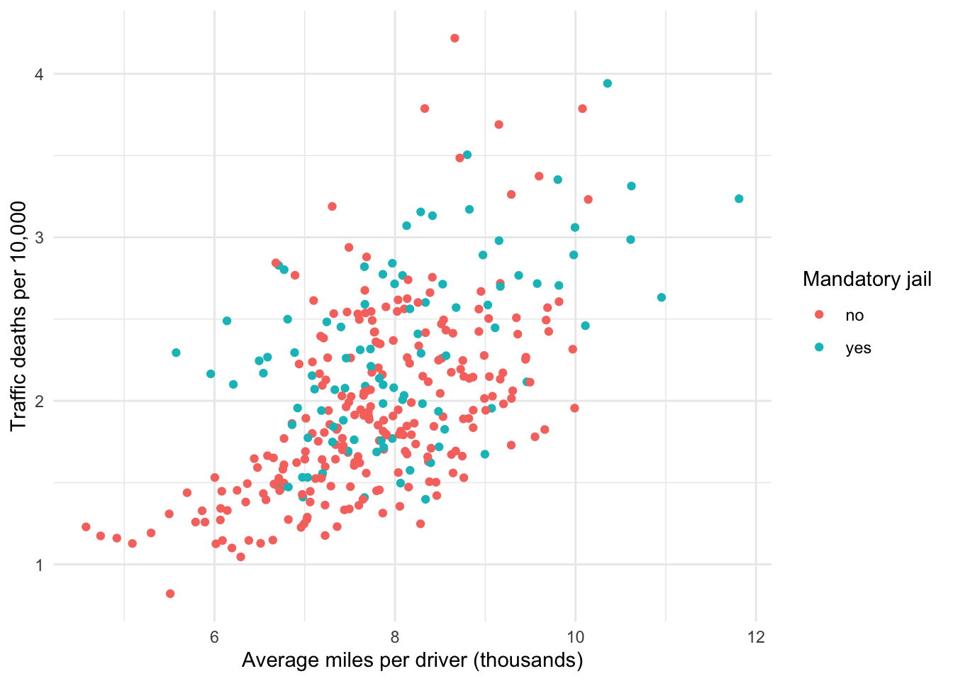
Figure 7.1: Relationship between miles driven and traffic fatalities
The exercise we just thought through is critical. Considering whether the slopes of our regression line should or do differ between categorical groups determines whether we should use the parallel slopes model or the interaction model. Which model is best to use is up to us to determine.
Why not simply add the interaction and if they are the same slope, so be it? Again, because we pay a penalty for adding superfluous explanatory variables. Also, an interaction model is more difficult to interpret and communicate to an audience. Most importantly, we should choose the model that reflects our theory based on our subject matter expertise.
Remember, choosing to use a parallel slopes model forces the slopes between groups to be drawn (i.e. estimated) as if they are parallel whether they actually are or not.
Let us now run the parallel slopes model, which generates the following results
| term | estimate | std_error | statistic | p_value | lower_ci | upper_ci |
|---|---|---|---|---|---|---|
| intercept | -0.238 | 0.182 | -1.304 | 0.193 | -0.597 | 0.121 |
| vmiles | 0.281 | 0.023 | 12.107 | 0.000 | 0.236 | 0.327 |
| jaild: yes | 0.265 | 0.056 | 4.726 | 0.000 | 0.155 | 0.376 |
Notice the variable name for the bottom row is
jaildyesand the estimate equals 0.265. This is the estimate for whenjaild = yes. There is no estimate forjaild = nobecause whenjaild = no, that is the same as \(d=0\) and so the estimate would simply be 0. Thejaildyesestimate is how states with a mandatory jail sentence compare to states without one.
Now we can plug our results into the sample regression equation to answer whatever questions we may have or encounter.
\[\begin{equation} \hat{mrall} = -0.238 + 0.281\times vmiles + 0.265 \times jaild \end{equation}\]
Compare this equation to Equations (7.2)-(7.5). The jaild variable is the \(d\) variable. It equals either 0 or 1. If a state does not have a mandatory jail sentence, then jaild = 0, and so we we would have as our regression equation
\[\hat{mrall} = -0.238 + (0.281\times vmiles) + (jaild \times 0)\]
\[\hat{mrall} = -0.238 + (0.281\times vmiles)\]
because, again, 0 multiplied by anything equals 0.
For states with a mandatory jail sentence, \(d=1\), and so we have as our regression equation
\[\hat{mrall} = -0.238 + (0.281 \times vmiles) + (0.265 \times 1)\]
Anything multiplied by 1 is equal to itself, so the above equation simplifies to
\[\hat{mrall} = -0.238 + (0.281 \times vmiles) + 0.265\]
And 0.265 is a constant number just like -0.238. These values can be combined.
\[\hat{mrall} = (-0.238 + 0.265) + (0.281\times vmiles)\]
And we can finally simplify the equation to look like the standard regression equation of \(\hat{y} = b_0 + b_1x\), but remember this is the equation for states with a mandatory jail sentence.
\[\hat{mrall} = 0.027 + (0.281\times vmiles)\]
And as a reminder, the equation for states without a mandatory jail sentence is
\[\hat{mrall} = -0.238 + (0.281\times vmiles)\]
The two regression lines have the same slope because we forced them to have the same slope. The only difference between the two regression lines is the y-intercept. Because \(b_2\), which in this example was
jaildyes, equals 0.265 as shown in Table 7.2, the intercept for states with a mandatory jail sentence is 0.265 higher than the intercept for states.
Figure 7.2 provides the same scatterplot but adds our parallel regression lines. Note that, as expected, the blue line is above the red line. Based on the results, we know the blue line is above the red line by 0.265. We also know that the slope for both lines is 0.281.

Figure 7.2: Parallel slopes visualization
When communicating an interpretation of the results for a parallel slopes model, we can write something like the following:
Controlling for whether a state has a mandatory jail sentence for drunk driving, the results indicate that as the average miles driven per driver in a state increases 1,000 miles, traffic fatalities per 10,000 population increase by 0.281, on average.
Why does the interpretation use an increase of 1,000 miles instead of 1 mile? Isn’t the estimate the predicted change in the outcome given a 1-unit increase in the explanatory variable? That is correct. However, remember that vmiles is in units of 1,000 miles. Imagine one state has a value of 6 and another of 7. That is a one unit increase for which the regression model estimates a predicted change in the traffic death rate. But this is not an increase of 1 mile, it is an increase of 1,000 miles; 6,000 to 7,000.
If we want to focus on the dummy variable, we could write:
On average, states with mandatory jail sentencing have a higher traffic fatality rate of 0.265 per 10,000, controlling for average miles driven per driver.
7.2.2 Beyond dummies
What if we want to include a categorical explanatory variable that has more than two levels? Doing so is easy and the logic works exactly the same as before. The only difference is that we use multiple dummy variables to represent the multiple levels of a categorical variable.
Suppose we included an explanatory variable with four levels instead of two. Such a variable can be represented in the regression equation like so:
\[\begin{equation} y = \beta_0 + \beta_1x + \beta_2d_1 + \beta_3d_2 + \beta_4d_3 + \epsilon \tag{7.7} \end{equation}\]
Just as we used one dummy variable to represent a categorical variable with two levels, we use three dummy variables to represent a categorical variable with four levels.
There is always one fewer dummy variables than there are levels of a categorical variable because one level must be used as the reference/base level to which all other levels are compared.
This model represented by Equation (7.7) draws four regression lines. One line for the group represented when \(d_1=0\), \(d_2=0\), and \(d_3=0\); a second line for the group represented when \(d_1=1\); a third line for the group represented when \(d_2=1\); and a fourth line for the group when \(d_3=1\). All the math demonstrated in the two-level case with Equations (7.2)-(7.5) works exactly the same way.
Let us apply this to our example. Suppose we were interested in whether traffic fatalities differ across U.S. regions. From the variables in Table 7.1, we might choose to construct the following model.
\[\begin{equation} mrall = \beta_0 + \beta_1vmiles + \beta_2region + \epsilon \tag{7.8} \end{equation}\]
where region is a four-level categorical variable containing South, West, N.East, and Midwest. Note that Equation (7.8) looks different than Equation (7.7). This is because Equation (7.8) leaves the various levels implied within the region variable. We can explicitly state the levels of region in our regression model instead, giving us
\[\begin{equation} mrall = \beta_0 + \beta_1vmiles + \beta_2d_{neast} + \beta_3d_{south} + \beta_4d_{west} + \epsilon \tag{7.9} \end{equation}\]
which now has the exact same structure as Equation (7.7). In this case, the Midwest level is excluded as the reference/base level. This is an arbitrary choice; we could choose to exclude any one of the levels to which all other levels are compared. Statistical software will automatically choose a default level. If the categorical variable is coded using text, then R excludes the level that comes first alphabetically. If coded numerically, one level should be coded as equal to 0 and will be the level that R excludes.
Figure 7.2 visualizes this model. Note that there are four regression lines, each corresponding to one of the four regions. There are clear differences between the regions. It appears states in the West and South are somehow different than states in the Midwest and Northeast with respect to traffic fatality rates.
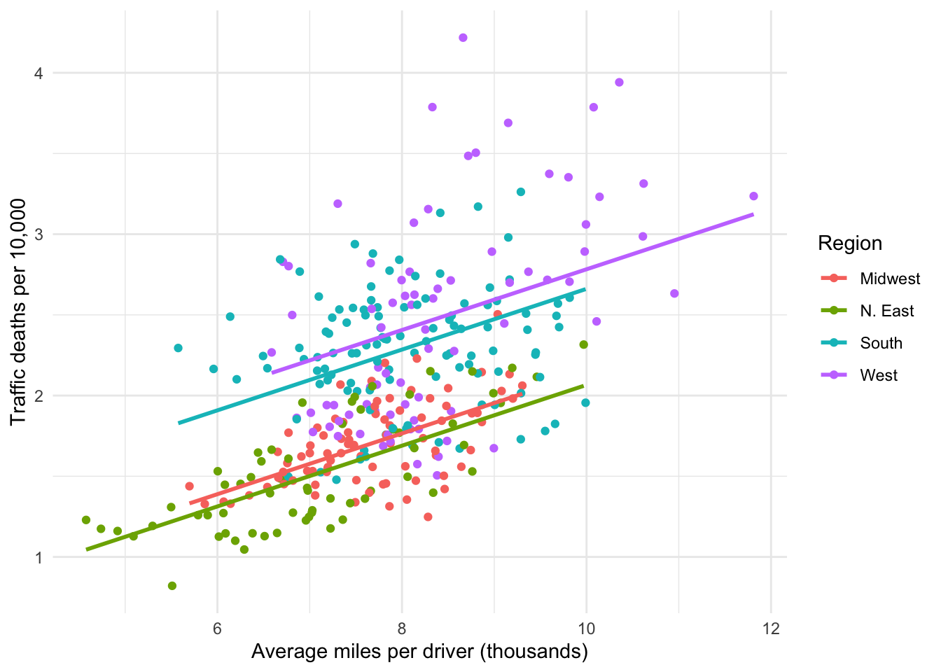
Figure 7.3: Parallel slopes for 4 groups
Running this model produces the following results.
| term | estimate | std_error | statistic | p_value | lower_ci | upper_ci |
|---|---|---|---|---|---|---|
| intercept | 0.260 | 0.167 | 1.553 | 0.121 | -0.069 | 0.589 |
| vmiles | 0.188 | 0.021 | 8.895 | 0.000 | 0.147 | 0.230 |
| region: N. East | -0.076 | 0.065 | -1.166 | 0.245 | -0.204 | 0.052 |
| region: South | 0.519 | 0.056 | 9.283 | 0.000 | 0.409 | 0.630 |
| region: West | 0.641 | 0.062 | 10.264 | 0.000 | 0.518 | 0.763 |
Note that Table 7.3 provides estimates for three of the four regions. This is no different from our previous model; jaild has two levels, yes and no, but Table 7.2 provides only one estimate for jaild=yes. No matter how many levels in a categorical variable, one of the levels is set such that \(d=0\) and so that level drops out of the equation.
Just like with the previous model where the estimate for
jaild=yesindicates how far above or below the regression line is relative to the line forjaild=no, the estimates for the three regions in Table 7.3 indicate how far above or below their respective regression lines are relative to the excluded level,region=Midwest.
In Table 7.3, Midwest is excluded as expected. We can plug our estimates into the sample version of Equation (7.9).
\[\hat{mrall} = 0.26 + (0.188 \times vmiles) + (-0.076 \times d_{neast}) + (0.519 \times d_{south}) + (0.641 \times d_{west})\]
For states in the Midwest, all three rightmost terms drop from the model because all of the \(d\) variables equal 0, leaving us with
\[\hat{mrall} = 0.26 + (0.188 \times vmiles)\]
For states in the N.East, \(d_{neast}=1\) and the other \(d\) variables equal 0, giving us
\[\hat{mrall} = 0.26 + (0.188 \times vmiles) + (-0.076 \times 1)\]
\[\hat{mrall} = (0.26 - 0.076) + (0.188 \times vmiles)\]
\[\hat{mrall} = 0.184 + (0.188 \times vmiles)\]
This means that states in the N.East have a lower traffic fatality rate than states in the Midwest, on average. How much lower? By the amount of the estimate associated with \(d_{neast}\): 0.076. This same process can be applied to the other two regions.
Look back at Figure 7.2, noting where the Midwest line is relative to the other regions. Northeast is below Midwest, while South and West are above it.
The estimates for the three included regions in Table 7.3 tell us how far the regions are above and below Midwest. Again, all regions have the same slope with respect to average miles driven because we forced them to be the same by using the parallel slopes model.
When communicating our results, we could write something like the following:
On average and controlling for average miles driven per driver, states in the Northeast region experience fewer traffic fatalities then state in the Midwest by approximately 0.08 per 10,000, while states in the South and West experience higher traffic fatality rates than states in the Midwest by 0.52 and 0.64, respectively.
7.3 Interaction model
What if we allowed the two slopes in Figure 7.2 to differ? If our expertise leads us to theorize the two slopes should differ between states with and without mandatory jail sentencing for drunk driving, and/or if visualizing the data suggests they do, then we can choose to use an interaction model.
Allowing the two slopes to differ means we allow the marginal effect of the average miles driven per driver to differ between the two groups of states.
Figure 7.4 visualizes this additional flexibility. Note that the slope of the red line is indeed slightly steeper than the blue line. Thus, this visualization suggests that average miles driven per mile in states without mandatory jail sentences for drunk driving increases the traffic fatality rate by slightly more than it does in states with a mandatory jail sentence.
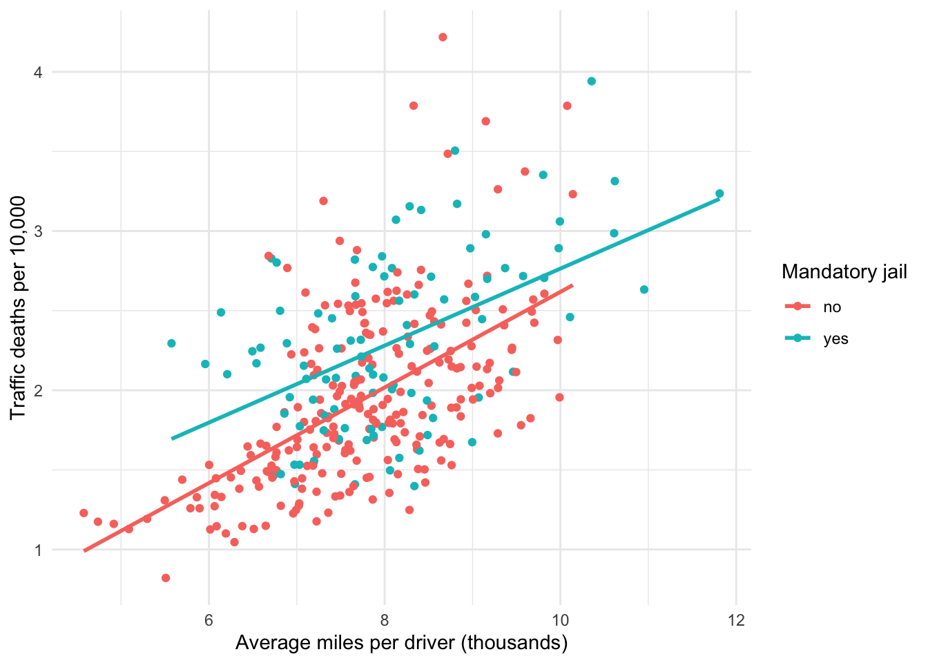
Figure 7.4: Interaction model visualization
This version of an interaction model involves interacting (i.e. multiplying) a categorical variable with a numerical variable. Equation (7.10) represents this version of the interaction model.
\[\begin{equation} y = \beta_0 + \beta_1x + \beta_2d + \beta_3xd + \epsilon \tag{7.10} \end{equation}\]
Equation (7.10) is similar to Equation (7.1) for the parallel slopes model. The difference is \(\beta_3xd\). This is the interaction–multiplying two of the explanatory variables in our regression model. Equation (7.11) provides the sample equation of this interaction model.
\[\begin{equation} \hat{y} = b_0 + b_1x + b_2d + b_3xd \tag{7.11} \end{equation}\]
Following the same process as with the parallel slopes model, we can rearrange Equation (7.11) to examine the logic of this interaction model. If \(d=0\), then \(b_2\) and \(b_3x\) drop out of the model because they are multiplied by 0. Thus, we have the same sample regression equation as Equation (7.3).
\[\begin{equation} \hat{y} = b_0 + b_1x \tag{7.12} \end{equation}\]
Equation (7.12) is the regression line for whatever group is represented when \(d=0\).
If \(d=1\), then \(b_2\) and \(b_3x\) remain in our model. As with the parallel slopes model, \(b_2\) combines with \(b_0\). This shifts the y-intercept for the group for which \(d=1\) either above or below the group for which \(d=0\) by the amount equal to \(b_2\). Because the lines are not parallel, just because a line starts above or below another does not mean it will stay above or below. It depends on the value of the \(b_3x\). The term \(b_3x\) is combined with \(b_1x\). Thus, if \(d=1\), we have the following sample regression equation
\[\begin{equation} \hat{y} = b_0 + b_1x + b_2d + b_3xd\\ \hat{y} = b_0 + b_1x + b_2 + b_3x\\ \hat{y} = (b_0 + b_2) + (b_1 + b_3)x \tag{7.13} \end{equation}\]
Equation (7.13) is the regression line for whatever group is represented when \(d=1\). This regression line will have an intercept above or below the regression line for which \(d=0\) by the amount \(b_2\), similar to the parallel slopes model. Critically, this regression line will also have a slope greater or lesser than the regression line for which \(d=0\) by the amount \(b_3\).
7.3.1 Using an interaction
Running this interaction model in our example produces the following results
| term | estimate | std_error | statistic | p_value | lower_ci | upper_ci |
|---|---|---|---|---|---|---|
| intercept | -0.384 | 0.221 | -1.741 | 0.083 | -0.819 | 0.050 |
| vmiles | 0.300 | 0.028 | 10.634 | 0.000 | 0.245 | 0.356 |
| jaild: yes | 0.731 | 0.399 | 1.831 | 0.068 | -0.054 | 1.516 |
| vmiles:jaildyes | -0.058 | 0.050 | -1.178 | 0.240 | -0.156 | 0.039 |
Once again, we can plug these values into Equation (7.11) to obtain the following regression equation
\[\hat{mrall} = -0.384 + (0.3\times vmiles) + (0.731\times jaild) + (-0.058\times vmiles \times jaild)\]
For states without mandatory jail sentencing (jaild = 0), the equation simplifies to
\[\hat{mrall} = -0.384 + 0.3\times vmiles\]
When communicating an interpretation of this equation, we might write something like:
For states that do not have a mandatory jail sentence for drunk driving, as the average miles driven per mile increases by 1,000 miles, traffic fatalities per 10,000 increases by 0.3, on average.
For states with mandatory jail sentencing (jaild = 1), the equation is
\[\hat{mrall} = -0.384 + (0.3\times vmiles) + (0.731\times jaild) + (-0.058\times vmiles \times jaild)\]
which simplifies to
\[\hat{mrall} = -0.384 + (0.3\times vmiles) + 0.731 + (-0.058\times vmiles)\]
which simplifies further to
\[\hat{mrall} = (-0.384 + 0.731) + (0.3-0.058)\times vmiles\]
and finally to
\[\hat{mrall} = 0.347 + 0.242\times vmiles\]
When communicating an interpretation of this equation, we might write something like:
For states that have a mandatory jail sentence for drunk driving, as the average miles driven per mile increases by 1,000 miles, traffic fatalities per 10,000 increases by 0.242, on average.
Look back at Figure 7.4. As we suspected the slope of the blue line that represents states with a mandatory jail sentence is less than the slope of the red line representing states without a mandatory jail sentence. How much less? By the amount of the estimate associated with the interaction term, vmiles:jaildyes in Table 7.4: 0.058.
The intercepts of the two lines are also different. If the x-axis in Figure 7.4 were extended to 0 and the regression lines were extrapolated to the left until they intersect the y-axis, the blue line would intersect at 0.347, while the red line would intersect at -0.384. Note that the difference between these two intercepts is the estimate associated with the dummy variable jaildyes in Table 7.4: 0.731.
This is a case where the intercept does not have a practical application because vmiles never equals 0, and even if it did, the predicted traffic fatality rate cannot be negative like the regression for states without mandatory sentencing would predict.
7.3.2 Variations
Variations on interaction models are beyond the scope of this book, but suffice it to say we can interact any two variables we deem necessary (or more). If you suspect that the effect of a variable on an outcome depends on the value of another variable, then an interaction is how to model such a relationship.
7.4 Linear probability model
We have now covered the inclusion of categorical variables on the explanatory side of a regression model. We can also include categorical variables as an outcome. In fact, many interesting question involve outcomes of a categorical nature, particularly binary. For example,
- Did the person graduate from college (yes or no)?
- Did the government default on its bond payments?
- Did the program participant get a job afterward?
- Did the nonprofit receive the grant it applied for?
As before, we may want to explain or predict such outcomes based on a set of explanatory variables.
A linear probability model (LPM) is just a special name we give the kind of regression we have already covered but when the outcome is a dummy variable instead of continuous. The key difference between an LPM and what we have already done concerns probability. Regression with a numerical outcome explains or predicts changes or values of the outcome in terms of the outcome’s units.
The LPM explains or predicts changes or values in the probability that the dummy outcome equals 1. If the dummy outcome is coded such that \(d=1\) means the event did occur, then the LPM estimates the change in or value of the probability that the event in question occurs given a change or value for the explanatory variable(s).
Equation (7.14) shows the generic population LPM, which is the same as the generic multiple regression population model except for the left-hand side. All this equation is trying to denote is that our estimates on the right-hand side pertain to the probability (Pr) that \(y=1\). Equation (7.15) shows the sample LMP equation.
\[\begin{equation} Pr(y=1)=\beta_0+\beta_1x_1+\beta_2x_2+\cdots+\beta_kx_k+\epsilon \tag{7.14} \end{equation}\]
\[\begin{equation} \hat{Pr(y=1)}=b_0+b_1x_1+b_2x_2+\cdots +b_kx_k \tag{7.15} \end{equation}\]
Again, nothing is different with respect to how we use the above equations to answer questions concerning the predicted change or value of the outcome. We simply need to remember that those changes or values will be expressed as probabilities that \(y=1\) and what it means for \(y\) to equal 1 in the context of our particular question.
7.4.1 Using LPM
What if instead of modeling traffic fatality rates as an outcome dependent on miles driven and mandatory jail sentencing for drunk driving, we modeled whether a state has mandatory sentencing as an outcome dependent on traffic fatality rates and region? Perhaps states passed such laws because they have high traffic fatality rates. Equation (7.16) represents our model in this case.
\[\begin{equation} Pr(jaild=1)=\beta_0+\beta_1vmiles+\beta_2region+\epsilon \tag{7.16} \end{equation}\]
Scatter plots for LPMs are not particularly useful for communicating to an audience, but they can provide insight to what it is we are trying to do with an LPM, if it is not yet clear. Figure 7.5 changes the coding of jaild from yes/no to 1/0 and plots it on the y axis against traffic fatality rates on the x axis. Regions are excluded for simplicity.
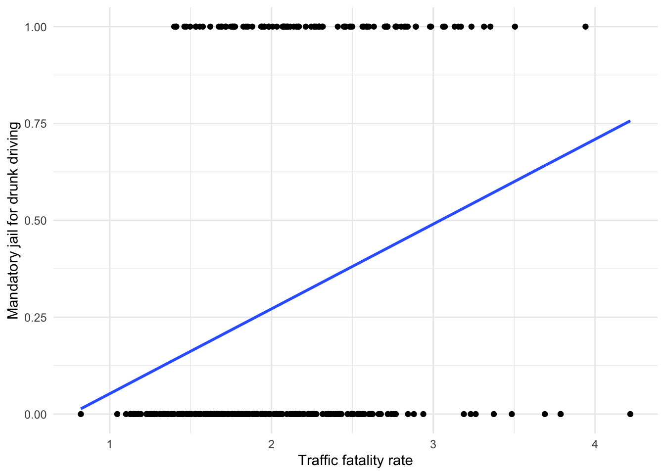
Figure 7.5: LPM visualization
Immediately, we should notice Figure 7.5 does not look like the typical scatter plots we have viewed thus far. This is because all observations fall into one of two values for jaild. It is also difficult to tell how our regression line is being drawn through the data.
The points along the x axis are states for which jaild = 0, meaning they do not impose mandatory jail sentencing for drunk driving. The points at the top are states for which jaild = 1. Compared to the points at the bottom, note the slight shift to the right the points at the top seem to have made. This shift is what informs the regression line to slope upward. The pattern of these data suggests there is a positive association between traffic fatality rate and passing a mandatory jail sentencing for drunk driving.
The values of \(y\) along the regression line are the predicted probabilities that a state has a mandatory jail law given the corresponding values for traffic fatality rate. For example, states with a rate of 3 appear to have a probability of 0.5 or 50% of passing a mandatory jail law.
Running this model produces the following results
| term | estimate | std_error | statistic | p_value | lower_ci | upper_ci |
|---|---|---|---|---|---|---|
| intercept | -0.066 | 0.102 | -0.645 | 0.520 | -0.267 | 0.135 |
| mrall | 0.117 | 0.054 | 2.171 | 0.031 | 0.011 | 0.222 |
| region: N. East | 0.064 | 0.070 | 0.913 | 0.362 | -0.074 | 0.202 |
| region: South | 0.040 | 0.068 | 0.580 | 0.562 | -0.094 | 0.173 |
| region: West | 0.361 | 0.078 | 4.634 | 0.000 | 0.208 | 0.514 |
Plugging these results into our sample regression equation gives us
\[\hat{Pr(jaild=1)}= -0.07 + (0.12 \times mrall) + (0.06 \times d_{neast}) + (0.04 \times d_{south}) + (0.36 \times d_{west})\]
Once again, we are back to plug-and-chug. For example, what is the predicted probability that a state in the Midwest with a traffic fatality rate of 2.5 has a mandatory jail sentence for drunk driving?
\[\hat{Pr(jaild=1)}= -0.07 + (0.12 \times 2.5)\]
\[\hat{Pr(jaild=1)}=0.23\]
There is a 23% likelihood that such a state has such a law.
How would an increase of 2 fatalities per 10,000 affect the probability that a state imposes a mandatory jail law?
\[\Delta \hat{Pr(jaild=1)}=0.12 \times 2\]
\[\Delta \hat{Pr(jaild=1)}=0.24\]
An increase in the traffic fatality rate of 2 is predicted to increase the probability that a state passes a mandatory jail sentence for drunk driving by about 24 percentage points.
Furthermore, our results suggest states in the West are substantially more likely to have this law. Compared to the Midwest, the West is 36 percentage points more likely to have a law and about 30 percentage points more likely than states in the South and Northeast.
7.4.2 Fit
Because our outcome is a dummy variable, it does not have the same kind of variation we need to assess model fit like before using \(R^2\) or RMSE. Since we are explaining or predicting whether or not an outcome occurs, we can assess the fit of the model based on how well it predicts the observed outcomes.
We could change this threshold, but suppose we decide that if our model predicts the likelihood of an outcome at 50% (0.50) or greater, then we say that our model predicts the outcome will occur \(y=1\) and \(y=0\) if our model predicts a likelihood less than 0.50. Table 7.6 shows a few rows applying this logic. Note that each row shows the observed data for each variable in our model, then the predicted probability in the jaild_hat column, then the rounding of that probability to 0 or 1 in the prediction column. Note the similarities and differences between the observed outcomes in jaild and the predicted outcomes prediction. Sometimes our model predicts correctly, and sometimes it does not.
| ID | jaild | mrall | region | jaild_hat | prediction |
|---|---|---|---|---|---|
| 29 | 0 | 2.174 | West | 0.549 | 1 |
| 113 | 1 | 1.461 | N. East | 0.169 | 0 |
| 254 | 0 | 0.821 | N. East | 0.094 | 0 |
| 98 | 1 | 1.936 | Midwest | 0.160 | 0 |
| 68 | 0 | 2.575 | West | 0.596 | 1 |
| 241 | 1 | 2.080 | West | 0.538 | 1 |
| 182 | 0 | 1.825 | N. East | 0.211 | 0 |
Table 7.7 below is referred to as a confusion matrix. It is simply a cross-tabulation of the observed outcomes and the predicted outcomes with the predictions along the top as columns.
| 0 | 1 | |
|---|---|---|
| 0 | 210 | 31 |
| 1 | 56 | 38 |
We can see that there are 248 cases where our model correctly predicts the outcome (210 + 38). There are 87 cases where our model incorrectly predicts the outcome. Specifically, there are 31 cases where our model predicts a state has a law but doesn’t and 56 cases where our model predicts a state does not have a law but does. We can also convert these to percentages like the table below. These confusion matrices help us assess and communicate how accurate our model is.
| 0 | 1 | |
|---|---|---|
| 0 | 0.79 | 0.45 |
| 1 | 0.21 | 0.55 |
To learn how to run the regression models from Chapters 6 and 7 in R, proceed to Chapter 21.