2 Data
Nothing exists except atoms and empty space; everything else is opinion.
—Democritus
Data are like the atoms of knowledge. We cannot effectively convert this raw material of knowledge into a useful product without first understanding the raw material. Therefore, learning statistics naturally begins with learning the types and structures of data.
2.1 Learning objectives
- Understand the organization of rectangular data
- Identify the unit of analysis within a dataset
- Identify and distinguish types of variables
- Identify and distinguish types of dataset structures
2.2 Rectangular Data
| Variable_1 | Variable_2 | Variable_3 |
|---|---|---|
| Datum (Unit of Analysis) | Datum | Datum |
| Datum (Unit of Analysis) | Datum | Datum |
| Datum (Unit of Analysis) | Datum | Datum |
Rectangular data is organized by rows and columns. A rectangular dataset has three components. Not all datasets will match the below description because datasets are not always organized correctly.
- Unit of analysis: The entity or subject a row of data refers to. The unit of analysis uniquely identifies each row of a dataset. If we have a dataset of 50 states and some variables measured in 2020, then our unit of analysis is states. If you were told a specific state, then you could find the row in the dataset. If we have 50 states measured in 2019 and 2020, then the unit of analysis is state-year because you will need to know the state and year to find a specific row.
- Variable: A measured characteristic of the unit of analysis. State unemployment rate is a variable for a state unit of analysis. In this example, state name is a variable as well as the unit of analysis.
- Datum: The intersection of a variable (column) and an observation (row) resulting in a cell. The datum is a particular piece of information. A cell could contain something like 4.8 as the unemployment rate for Georgia in 2020.
2.3 Types of variables
The variables in a given dataset can be of several types. Types of variables are important to learn because it has consequences for data applications, such as description, visualization, and inference. Different types of variables offer different levels of information.
For example, suppose you ask two people to report their annual income. What options do they have for answers? If virtually any value, then you know to a precise degree the income each earns and can compute the precise difference between the two incomes. What if their choices are either more or less than $50,000? Then, you have a coarse understanding of how much they earn. If they provide different answers, you can only conclude whether one makes more than the other but not by how much. If they provide the same answer, then the two are grouped together even though it is highly unlikely they earn equal incomes. This makes a serious difference for statistical analysis.
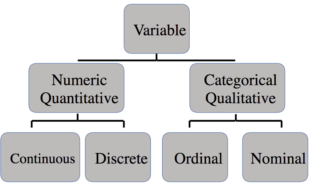
Figure 2.1: Variable Types
All variables belong to one of two broad types: qualitative (categorical) or quantitative (numeric).
- Qualitative variables take on values that have no intrinsic numerical meaning. They are naturally expressed in words.
- Quantitative variables take on values that do have intrinsic numerical meaning. They are naturally expressed using numbers.
2.3.1 Qualitative variables
Qualitative variables can be further differentiated into two types: nominal and ordinal.
- Nominal variables take on values that differ in name only. There is no way to rank a value as more or less than another value.
- Ordinal variables take on values that can be ranked relative to each other but the difference between rankings has no numerical value.
The values that categorical variables take on are commonly referred to as levels. Categorical variables can contain virtually any number of levels, though the number of levels is usually limited.
If our unit of analysis is individuals, a variable such as assigned sex contains two levels: male and female. The variable sex is nominal because its values have no numerical meaning and the two levels have no ranking. Race, state, country, continent, political party, and any variable coded as yes/no such as unemployed, married, or participated in some program are all examples of nominal variables.
If you have ever participated in a customer satisfaction survey, then you have contributed data to an ordinal variable. Those scales that provide some number of options from “disagree” to “agree” are called Likert scales. Your answer has no intrinsic numerical value but it can be ranked against the answers of others. One respondent can be said to be more satisfied than another but not by how much. Moreover, one can only trust the results insofar as respondents have the same understanding or frame of reference–the service that satisfied one respondent may not have satisfied another. Other ordinal variables for which there is a commonly understood scale, such as education level (high school, associate, bachelor, post-graduate) and income level (more or less than the federal poverty line) do not have this issue.
Qualitative variables can be aggregated to a higher unit of analysis such that they become quantitative variables. For example, the U.S. Census records race at the individual level (nominal). This information is then used to report the percentage of a state’s population by race, such as Georgia’s population being about 32% Black or African American. What is categorical variable at the individual level is now a quantitative variable at the state level.
2.3.2 Quantitative variables
Quantitative variables can be further differentiated into two types: discrete and continuous.
- Discrete variables take on countable or indivisible values.
- Continuous variables take on infinitely divisible values (at least in theory).
Any variable that is a count of persons, places, events, or things is a discrete variable, taking on integer values (e.g. 0, 1, 2, 3,…). The count of homeless people in a city, students in a classroom, hospital beds, or nonprofit volunteers are all discrete variables.
Many discrete variables can be treated as if continuous without any consequences. All of the examples above could likely be treated as conitnuous in an analysis.
When should we care that a variable is discrete? Chapter 4 and chapters on inference will discuss how statistics relies heavily on the normal distribution, also referred to as a bell curve. If a discrete variable can take on integer values only, and especially if only a few values are possible, then that variable is unlikely to be normally distributed.
Rare discrete events, such as plane crashes or government defaults are not normally distributed. Application of basic statistical procedures to such variables may be inappropriate, requiring methods outside to scope of this course.
In many cases, if a variable is numeric, then it is continuous or can be treated as such. Continuous variables can contain values with an infinite number of decimal places. Still, continuous variables are recorded in data with a limited number of decimal places because either we measure phenomena with finite precision or it simply becomes impractical to include so many decimal places. For example, age is usually recorded in discrete years, but we could record continuously to the zeptosecond (a trillionth of a billionth of a second).
Many discrete variables become continuous because we calculate averages, proportions, or rates from them.
The number of students in the classroom is discrete (e.g. 20, 25, etc.), but the average number of students in classrooms (i.e. total students/number of classrooms) is continuous. This is how we can have values such as 22.5 for pupil-to-teacher ratio. The number of homeless people in a city is discrete but the proportion of the city’s population that is homeless (count of homeless/population) is continuous.
2.3.3 Index variables
Index variables can be ordinal or (usually) numerical but warrant separate discussion.
An index variable is a composite measure of multiple variables.
They can be used to make a continuous variable out of multiple categorical variables or simplify multiple quantitative variables into one quantitative measure. Purposes such as ranking colleges, measuring multidimensional poverty (i.e. factors beyond income), and determining political ideology make use of index variables.
Index variables mask underlying information. This can be helpful or harmful. In either case, it is important to consider how an index variable is constructed. Doing so can offer insight or uncover problems. An instructive example familiar to readers is college rankings. U.S. News and World Report describes how rankings are determined.
What makes a college good? According to these rankings, five percent of what makes a college good is the percent of undergraduate alumni giving a donation as a proxy of student satisfaction. Another 20% is based on the opinions of administrators at peer institutions. Are these choices wise? This is difficult to say and besides the point. The point is that index variables involve choices made by people and are not data that are observed directly. They are synthetic materials of knowledge and warrant careful consideration.
2.4 Dataset structures
Just as the type of variable one is dealing with impacts the kinds of visualizations or analyses one should use, so too does the structure of a dataset. Datasets come in three varieties depending on their unit of analysis.
- Cross-sectional
- Pooled cross-sectional
- Time series
- Panel or longitudinal
Cross-sectional data is a snapshot in time measuring some size sample of units. One column serves as the identifier of the unit of analysis, such as the name or ID number of the unit. Notice in Table 2.2 that all one needs to know is the country in order to identify a specific row.
| country | continent | year | lifeExp | pop | gdpPercap |
|---|---|---|---|---|---|
| Argentina | Americas | 2007 | 75.320 | 40301927 | 12779.380 |
| Bolivia | Americas | 2007 | 65.554 | 9119152 | 3822.137 |
| Brazil | Americas | 2007 | 72.390 | 190010647 | 9065.801 |
Pooled cross-sectional data could be considered a fourth structure but is simply multiple cross-sections stacked atop each other. The critical quality of pooled cross-sectional data is that each cross-section contains different units measured at different times, not the same units measured at different times. Notice in Table 2.3 that the countries included from 2002 are not the same as those included from 2007.
| country | continent | year | lifeExp | pop | gdpPercap |
|---|---|---|---|---|---|
| Algeria | Africa | 2002 | 70.994 | 31287142 | 5288.040 |
| Angola | Africa | 2002 | 41.003 | 10866106 | 2773.287 |
| Benin | Africa | 2002 | 54.406 | 7026113 | 1372.878 |
| Botswana | Africa | 2002 | 46.634 | 1630347 | 11003.605 |
| Argentina | Americas | 2007 | 75.320 | 40301927 | 12779.380 |
| Bolivia | Americas | 2007 | 65.554 | 9119152 | 3822.137 |
| Brazil | Americas | 2007 | 72.390 | 190010647 | 9065.801 |
Time series data measures one unit over multiple time periods. The unit of analysis in time series data is time, as it uniquely identifies each row. Notice in Table 2.4 that one country is tracked over multiple years.
| country | continent | year | lifeExp | pop | gdpPercap |
|---|---|---|---|---|---|
| Argentina | Americas | 1977 | 68.481 | 26983828 | 10079.027 |
| Argentina | Americas | 1982 | 69.942 | 29341374 | 8997.897 |
| Argentina | Americas | 1987 | 70.774 | 31620918 | 9139.671 |
| Argentina | Americas | 1992 | 71.868 | 33958947 | 9308.419 |
| Argentina | Americas | 1997 | 73.275 | 36203463 | 10967.282 |
| Argentina | Americas | 2002 | 74.340 | 38331121 | 8797.641 |
| Argentina | Americas | 2007 | 75.320 | 40301927 | 12779.380 |
Panel (or longitudinal) data measures the same units over multiple time periods. The unit of analysis is pair of unit and time period. Notice in Table 2.5 that in order to identify a specific row, you would need to know the country and year. One could also think of panel data as numerous time series.
| country | continent | year | lifeExp | pop | gdpPercap |
|---|---|---|---|---|---|
| Argentina | Americas | 1997 | 73.275 | 36203463 | 10967.282 |
| Argentina | Americas | 2002 | 74.340 | 38331121 | 8797.641 |
| Argentina | Americas | 2007 | 75.320 | 40301927 | 12779.380 |
| Bolivia | Americas | 1997 | 62.050 | 7693188 | 3326.143 |
| Bolivia | Americas | 2002 | 63.883 | 8445134 | 3413.263 |
| Bolivia | Americas | 2007 | 65.554 | 9119152 | 3822.137 |
To learn how to examine data in R, proceed to Chapter 17.